Week 3.5 - Deriving 4th order approximation of a 2nd order derivative using Taylor Table method
Aim: Derive the following 4th order approximations of the second-order derivative.
1. Central difference
2. Skewed right-sided difference
3. Skewed left-sided difference
Solution:
CENTRAL DIFFERENCING SCHEME:
NO OF NODES:
The number of nodes = p+q-1
Where, p is order of derivative.
q is order of approximations.
The no of nodes = 2+4-1 =>5.
DERIVATION:
To derive a fourth order approximation for the second order derivative,we start with these approximation,
`(∂^ 2 u)/( ∂ x^ 2) = [a f ( i − 2 ) + b f ( i − 1 ) + c f ( i ) + d f ( i + 1 ) + e f ( i + 2 )]/ (d x ^2)`-------(1)
taylor series derivation for the above terms,
`a f ( i − 2 ) = a f ( i ) − (2 a f ' ( i ) d x)/ (1 !) + (4 a f ' ' ( i ) d x^ 2)/( 2 !) + (8 a f ' ' ' ( i ) d x^ 3)/( 3 !) + (16 a f ' ' ' ' ( i ) d x^ 4)/( 4 !)`
Simillarly expand all the terms in the equation (1) and are represented in the form of table using taylor table method.
| dx^2f′′(i) | f(i) | f'(i)dx | f''(i)dx^2 | f'''(i)dx^3 | f''''(i)dx^4 |
| af(i-2) | a | -2a | 2a | −4a/3 | 2a/3 |
| bf(i-1) | b | -b | b/2 | −b/6 | b/24 |
| cf(i) | c | 0 | 0 | 0 | 0 |
| df(i+1) | d | d | d/2 | d/6 | d/24 |
| ef(i+2) | e | 2e | 2e | 4e/3 | 2e/3 |
| sum of co_efficients | 0 | 0 | 1 | 0 | 0 |
the linear equation obtained from the above table are solved using matrix inversion method,
A.X = B
on solving we get the coefficient as shown below,
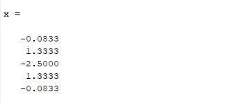
SKEWED RIGHT HAND DIFFERENCE SCHEME:
NO OF NODES:
The number of nodes = p+q
Where, p is order of derivative.
q is order of approximations.
The no of nodes = 2+4 =>6.
DERIVATION:
To derive a fourth order approximation for the second order derivative,we start with these approximation,
`(∂^ 2 u)/( ∂ x ^2) = [a f ( i ) + b f ( i + 1 ) + c f ( i + 2 ) + d f ( i + 3 ) + e f ( i + 4 ) + g f ( i + 5 )]/ (d x ^2)`
expand all the terms in the equation above
| dx^2f''(i) | f(i) | f'(i)dx | f''(i)dx^2 | f'''(i)dx^3 | f''''(i)dx^4 |
| af(i) | a | 0 | 0 | 0 | 0 |
| bf(i+1) | b | b | b/2 | b/6 | b/24 |
| cf(i+2) | c | 2c | 4c/2 | 8c/6 | 16c/24 |
| df(i+3) | d | 3d | 9d/2 | 27d/6 | 81d/24 |
| ef(i+4) | e | 4e | 16e/2 | 64e/6 | 256e/24 |
| gf(i+5) | g | 5g | 25g/2 | 125g/6 | 625g/24 |
the linear equation obtained from the above table are solved using matrix inversion method,
A.X = B
on solving we get the coefficient as shown below,
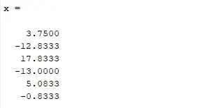
SKEWED LEFT HAND DIFFERENCE SCHEME:
NO OF NODES:
The number of nodes = p+q
Where, p is order of derivative.
q is order of approximations.
The no of nodes = 2+4 =>6.
DERIVATION:
To derive a fourth order approximation for the second order derivative,we start with these approximation,
`(∂^ 2 u)/( ∂ x^ 2) = [a f ( i − 5 ) + b f ( i − 4 ) + c f ( i − 3 ) + d f ( i − 2 ) + e f ( i − 1 ) + g f ( i )] /(dx ^2)`
expand all the terms in the equation above using taylor series expansion and are represented in the form of table using taylor table method.
| dx^2f''(i) | f(i) | f'(i)dx | f''(i)dx^2 | f'''(i)dx^3 | f''''(i)dx^4 | f'''''(i)dx^5 |
| af(i-5) | a | -5a | 25a/2 | −125a/6 | 625a/24 | −3125a/120 |
| bf(i-4) | b | -4b | 16b/2 | −64b/6 | 256b/24 | −1024b/120 |
| cf(i-3) | c | -3c | 9c/2 | −27c/6 | 81c/24 | −243c/120 |
| df(i-2) | d | -2d | 4d/2 | −8d/6 | 16d/24 | −32d/120 |
| ef(i-1) | e | -e | e/2 | −e/6 | e/24 | −e/120 |
| gf(i) | g | 0 | 0 | 0 | 0 | 0 |
| sum of co_efficients | 0 | 0 | 1 | 0 | 0 | 0 |
the linear equation obtained from the above table are solved using matrix inversion method,
A.X = B
on solving we get the coefficient as shown below,
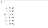
FUNCTION CODE FOR CENTRAL DIFFERENCING:
function Error_central_differencing = fourth_order_central_differencing(x,dx)
% analytic function = exp(x)*cos(x)
% analytic derivative
%f''(x) = -2*exp(x)*sin(x)
analytical_derivative = -2*exp(x)*sin(x);
%numerical derivative
%central differencing
central_differencing = (((-0.0833)*((exp(x-(2*dx)))*(cos(x-(2*dx)))))+((1.3333)*((exp(x-dx))*(cos(x-dx))))-((2.5000)*((exp(x))*(cos(x))))+((1.3333)*((exp(x+dx))*(cos(x+dx))))-((0.0833)*((exp(x+(2*dx)))*(cos(x+(2*dx))))))/(dx^2);
%error
Error_central_differencing = abs(central_differencing- analytical_derivative);
end
FUNCTION CODE FOR SKEWED RIGHT SIDED DIFFERENCE:
function Error_right_sided_skew = fourth_order_right_sided_skew(x,dx)
% analytic function = exp(x)*cos(x)
% analytic derivative
%f''(x) = -2*exp(x)*sin(x)
analytical_derivative = -2*exp(x)*sin(x);
%numerical derivative
%central differencing
right_sided_skew = (((3.7500)*((exp(x))*(cos(x))))-((12.8333)*((exp(x+dx))*(cos(x+dx))))+((17.8333)*((exp(x+(2*dx)))*(cos(x+(2*dx)))))-((13.0000)*((exp(x+(3*dx)))*(cos(x+(3*dx)))))+((5.0833)*((exp(x+(4*dx)))*(cos(x+(4*dx)))))-((0.8333)*((exp(x+(5*dx)))*(cos(x+(5*dx))))))/(dx^2);
%error
Error_right_sided_skew = abs(right_sided_skew- analytical_derivative);
end
FUNCTION CODE FOR SKEWED LEFT SIDED DIFFERENCE:
function Error_left_sided_skew = fourth_order_left_sided_skew(x,dx)
% analytic function = exp(x)*cos(x)
% analytic derivative
%f''(x) = -2*exp(x)*sin(x)
analytical_derivative = -2*exp(x)*sin(x);
%numerical derivative
%central differencing
left_sided_skew = (((-0.8333)*((exp(x-(5*dx)))*(cos(x-(5*dx)))))+((5.0833)*((exp(x-(4*dx)))*(cos(x-(4*dx)))))-((13.0000)*((exp(x-(3*dx)))*(cos(x-(3*dx)))))+((17.8333)*((exp(x-(2*dx)))*(cos(x-(2*dx)))))-((12.8333)*((exp(x-dx))*(cos(x-dx))))+((3.7500)*((exp(x))*(cos(x)))))/(dx^2);
%error
Error_left_sided_skew = abs(left_sided_skew- analytical_derivative);
end
Main Matlab Script:
clear all
close all
clc
x= pi/3;
dx= linspace(pi/4,pi/4000,20);
for i=1:length(dx)
central_differencing(i) = fourth_order_central_differencing(x,dx(i));
right_sided_skew(i) = fourth_order_right_sided_skew(x,dx(i));
left_sided_skew(i) = fourth_order_left_sided_skew(x,dx(i));
end
%plot
figure(1)
loglog(dx,central_differencing,'r')
hold on
loglog(dx,right_sided_skew,'g')
hold on
loglog(dx,left_sided_skew,'b')
xlabel('range of dx')
ylabel('truncation error')
title('range of dx vs error')
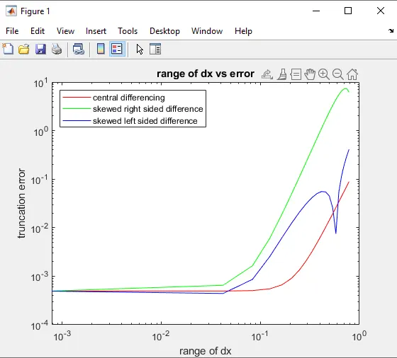
legend('central differencing','skewed right sided difference','skewed left sided difference','location','northwest')
Results: