Week 3 - Solving second order ODEs

Simple Pendulum

Aim:

Solving a second order ordinary differential equation of simple pendulum.

Objective:

• To convert second order ordinary differential equation to 1^st order ordinary differential equation.
• To create the function using python in-built function for solving ordinary differential equation.
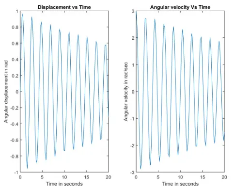
• To plot the displacement and velocity damping through the time stipulated time of simulation.

Description & Governing equation.

The differential equation is mostly used to define the complex physics phenomenon in the mathematical way. Differential equation is divided in two different classify as ordinary differential equation and partial differential equation. Solving a 1^st order differential is quite easy and require only one constant to define the equation, also it can be also programmed easily. The main effort is taken while solving 2^nd order differential equation. Most of the fluid equation and some structural phenomenon are defined in the 2^nd order differential equation which need to solve eventually to simulated the flow or study the structural behavior.

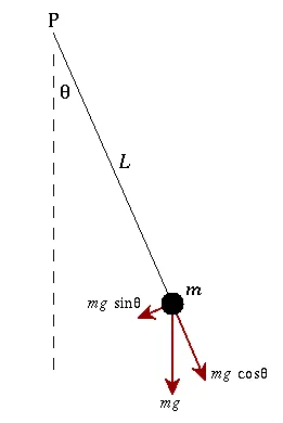
A simple pendulum consists of mass which is attached by the string of length L from a pivot point P. when displaced by initial force the mass gets moved back and forth performing periodic motion. By applying the Newton’s second law motion we can obtain the equation of motion for simple pendulum which is given as:

`(d^2 θ)/dt+b/m dθ/dt+g/L sinθ= 0`

To solve the equation in the MATLAB by using ‘ode45’ the equation needs to be converted from 2^nd order partial differential equation to 1^st order differential equation.

`Consider θ=θ1`

Then new equation of motion can be written as:

`(d^2 θ1)/(dt^2 )+b/m (dθ1)/(dt) +g/L sin⁡θ1 =0`

Consider,

`(dθ1)/dt=θ2`

Therefore, new equation can be written as:

`(dθ2)/dt+b/m θ2+g/L sin⁡θ1=0`

Which leads to:

`(dθ2)/dt= -b/m θ2-g/L sin⁡θ1`

The resultant first order equation will be:

`θ_1^'=θ2 and θ_2^'= -b/m θ2-g/L sin⁡θ1`

Code:

import numpy as np 
from scipy.intergate import odeint
import matplotlib.pyplot as plt 
import math

def model(theta,t,b,g,l,m):
	theta1 = theta[0]
	theta2 = theta[1]
	dtheta1_dt = theta2
	dtheta2_dt = -(b/m)*theta2 - (g/l)*math.sin(theta1)
	dtheta_dt = [dtheta1_dt,dtheta2_dt]
	return dtheta_dt

l = 1
m = 1
b = 0.05
g = 9.81

#initial
theta_0 = [0,3]

#time array
t = np.linspace(0,20,100)

#solution
theta = odeint(model,theta_0,t,args = (g,b,l,m))

#results
plt.plot(t,theta[:,0])
plt.plot(t,theta[:,1])
plt.show()

Results: