Project 2 - Rankine cycle Simulator

Aim:

• Create a Rankine Cycle Simulator using MATLAB
• Calculate the state points of the Rankine Cycle based on user inputs.
• Extracting steam and water properties from given file.
• Plot the corresponding T-s and h-s plots for the calculated state points.

Rankine cycle:

The Rankine cycle is the process widely used by power plants such as coal-fired power plants or nuclear reactors. In this mechanism, a fuel is used to produce heat within a boiler, converting water into steam which then expands through a turbine producing useful work.

Process 1: Isentropic compression in pump.

Process 2: Constant pressure heat addition in boiler.

Process 3: Isentropic expansion in turbine.

Process 4: Constant pressure heat rejection in condenser.

Program:

clear all
close all
clc

%taking input from user
p3=input('enter the pressure at turbine inlet:');
t3=input('enter the temperature at turbine inlet:');
p4=input('enter the pressure at condenser inlet:');

%from here we started calculating state point values

p1=p4;
p2=p3;
t5=XSteam('tsat_p',p3);
s5=XSteam('sL_p',p3);
t6=t5;
s6=XSteam('sV_p',p3);
h3=XSteam('h_pt',p3,t3);
s3=XSteam('s_pt',p3,t3);
s4=s3;
sf4=XSteam('sL_p',p4);
sv4=XSteam('sV_p',p4);
hf4=XSteam('hL_p',p4);
hv4=XSteam('hV_p',p4);
X4=(s3-sf4)/(sv4-sf4);
h4=hf4+(X4*(hv4-hf4));
h1=hf4;
s1=XSteam('sl_p',p4);
s2=s1;
v1=XSteam('vl_p',p4);

%work consumed by pump
work_of_pump=v1*(p3-p4)*100;
h2=h1+work_of_pump;

%work produced by turbine
work_of_turbine=h3-h4;

%net work output
net_work_output=work_of_turbine-work_of_pump;

%heat added in boiler at constant pressure
heat_added_in_boiler=h3-h2;

%heat rejected in condenser at constant pressure
heat_rejected_in_condenser=h4-h1;
t1=XSteam('tsat_p',p4);
cp=XSteam('cp_ps',p3,s2);
cv=XSteam('cv_ps',p3,s2);
k=cp/cv;
t2=t1*(p3/p4)^((k-1)/k);
t4=t1;

%calculating efficiency of rankine cycle and S.S.C
efficiency=net_work_output/(h3-h2);
Specific_steam_consumption=3600/net_work_output;
T=linspace(1,500,1000);
for i=1:length(T)
sf(i)=XSteam('sL_T',T(i));
sg(i)=XSteam('sV_T',T(i));
hf(i)=XSteam('hL_T',T(i));
hg(i)=XSteam('hV_T',T(i));
end

%here we have comlpete information of all state points

%now we start to plot graph for the calculated state points

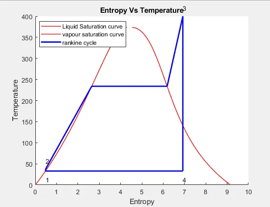
%figure1 is entropy Vs temperature plot

figure(1)
hold on
plot(sf,T,'r','linewidth',1)
plot(sg,T,'r','linewidth',1)
plot([s1 s2],[t1 t2],'b','linewidth',2)
plot([s2 s5],[t2 t5],'b','linewidth',2)
plot([s5 s6],[t5 t6],'b','linewidth',2)
plot([s6 s3],[t6 t3],'b','linewidth',2)
plot([s3 s4],[t3 t4],'b','linewidth',2)
plot([s4 s1],[t4 t1],'b','linewidth',2)
text(s1,t1-20,'1')
text(s2,t2+20,'2')
text(s3,t3+20,'3')
text(s4,t4-20,'4')
xlabel('Entropy')
ylabel('Temperature')
title('Entropy Vs Temperature')
legend('Liquid Saturation curve','vapour saturation curve','rankine cycle')

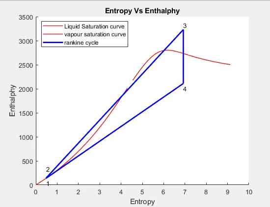
%figure2 is entropy Vs enthalphy plot

figure(2)
hold on
plot(sf,hf,'r','linewidth',1)
plot(sg,hg,'r','linewidth',1)
plot([s1 s2],[h1 h2],'b','linewidth',2)
plot([s2 s3],[h2 h3],'b','linewidth',2)
plot([s3 s4],[h3 h4],'b','linewidth',2)
plot([s4 s1],[h4 h1],'b','linewidth',2)
text(s1,h1-100,'1')
text(s2,h2+200,'2')
text(s3,h3+100,'3')
text(s4,h4-100,'4')
xlabel('Entropy')
ylabel('Enthalphy')
title('Entropy Vs Enthalphy')
legend('Liquid Saturation curve','vapour saturation curve','rankine cycle')

%from here we start displaying all state points and other useful information that we have calculated.

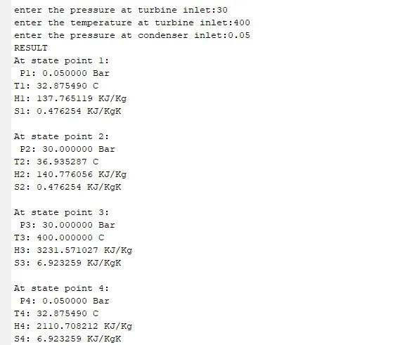
disp('RESULT')
fprintf('At state point 1:\n ');
fprintf('P1: %f Bar\n',p1);
fprintf('T1: %f C\n',t1);
fprintf('H1: %f KJ/Kg\n',h1);
fprintf('S1: %f KJ/KgK\n',s1);
fprintf('\n')
fprintf('At state point 2:\n ');

fprintf('P2: %f Bar\n',p2);
fprintf('T2: %f C\n',t2);
fprintf('H2: %f KJ/Kg\n',h2);
fprintf('S2: %f KJ/KgK\n',s2);
fprintf('\n')
fprintf('At state point 3:\n ');
fprintf('P3: %f Bar\n',p3);
fprintf('T3: %f C\n',t3);
fprintf('H3: %f KJ/Kg\n',h3);
fprintf('S3: %f KJ/KgK\n',s3);
fprintf('\n')
fprintf('At state point 4:\n ');
fprintf('P4: %f Bar\n',p4);
fprintf('T4: %f C\n',t4);
fprintf('H4: %f KJ/Kg\n',h4);
fprintf('S4: %f KJ/KgK\n',s4);
fprintf('\n')
fprintf('Turbine work: %f KJ/Kg\n',work_of_turbine);
fprintf('Pump work: %f KJ/Kg\n',work_of_pump);
fprintf('Wnet: %f KJ/Kg\n',net_work_output);
fprintf('Efficiency: %f Percent\n',efficiency);
fprintf('S.S.C: %f KJ/KWh\n',Specific_steam_consumption);

%%%%%%%%%%%%%%%%%%%%%%%%%%%%%%%%%%%%%%%%%%%%%%%%%%%%%%%%%%%%%%%%%%%%%%%%%%%%%%%%%%%%%%%%%%%%%%%%%%%%%%

Output:

Plots:

Results: