MIXING EFFICIENCY PROJECT

Aim: This project aims to study the thermal mixing in tee junction using the finite volume method and understand the use of the k-ꙍ SST and k-Ꜫ turbulence models.

Introduction

In this project, steady-state simulations are set up to compare the mixing effectiveness when the hot inlet is at a temperature of 36°C and the cold inlet is at a temperature at 19°C in ANSYS Fluent. k-ꙍ SST and k-Ꜫ turbulence models are firstly implemented and the most suitable model is chosen. Then phenomenon of thermal mixing is being investigated for further two different testcase scenarios. The first testcase comprises a short mixing tee model with a hot inlet velocity of 3m/s and two different momentum ratios of 2,4. The second testcase comprises a long mixing tee model with the same hot inlet velocity and momentum ratios. The detailed mesh and setup parameters used for CFD simulations are described and the results of both cases are compared. And based on that comparison, conclusions are made.

Theory:

The study of fluid mixing at different temperatures in geometries such as tee junction is of significant importance since it finds its applications in various fields such as thermal striping and thermal fatigue problems in nuclear power plants.

Problem Description

Throughout our study, the specifications for the geometry as well as the fluid used are as follow:

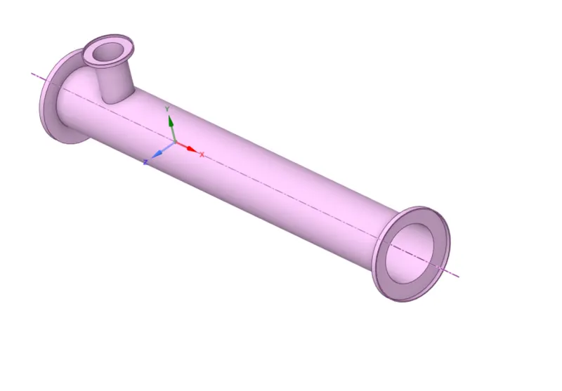
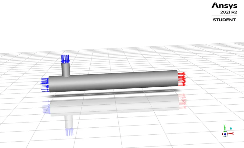
• The geometries used are that of two crossing pipes forming T-junction as shown below.
• For the long mixing tee as well as short mixing tee, the radius of the hot inlet is R1=17.44mm; the radius at the cold inlet is R2=8.98mm and the radius at the outlet being equal to R1. The length of the short mixing tee is L1=191mm and the length of the long mixing tee is L2=267.33mm.
• The fluid used is Air (`ρ=1.225kg/m^3 ,μ=1.784×10^(-4) kg/ms`) enters the computational domain through the hot inlet (R1) at u1=3m/s. The inlet velocity at R2 is computed using momentum ratios 2,4 for both short and long mixing tee. That implies u2=6 & 12m/s respectively.
• Boundary conditions used:

-Velocity-inlet at different inlets

-Pressure-outlet at the outlet

-Wall for the surface of the volume

• Steady-state simulation is performed using Ansys Fluent with the pressure-based coupled solver.

Methodology:

In order to carry our study, several steps are involved:

• The first step is about the choice of the suitable turbulence model between k-ꙍ SST and k-Ꜫ turbulence models; so, to run the case which allows us to achieve this the fluid volume is extracted from the given geometry in
• After this, the resulting volume is discretized under Mesh module and different boundary surfaces are named accordingly.
• Now the appropriate computational domain is applied along with turbulence models and energy equations.
• To sum up the hole process, the base testcase is run to choose the suitable turbulence model; After that the suitable grid size is chosen by performing grid independence test.
• Simulations are run and effect of momentum ratios as well as the geometry length is noted. And finally, inferences are made to find areas of improvement if any.

Pre-processing

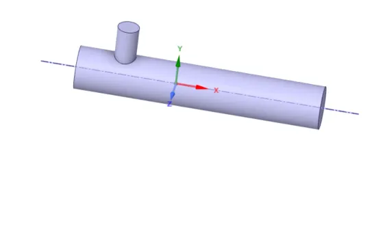
As described a bit above, the CAD model is imported in Spaceclaim where the wet volume is extracted as shown below.

Now, moving to the mesh module, the computational domain is defined. According to the boundary conditions, the hot inlet is named as ‘inlethotx’ and the cold inlet is named as ‘inletcoldy’. The external sufaces of the volume are named as ‘Walls’. The outlet keeping its name.

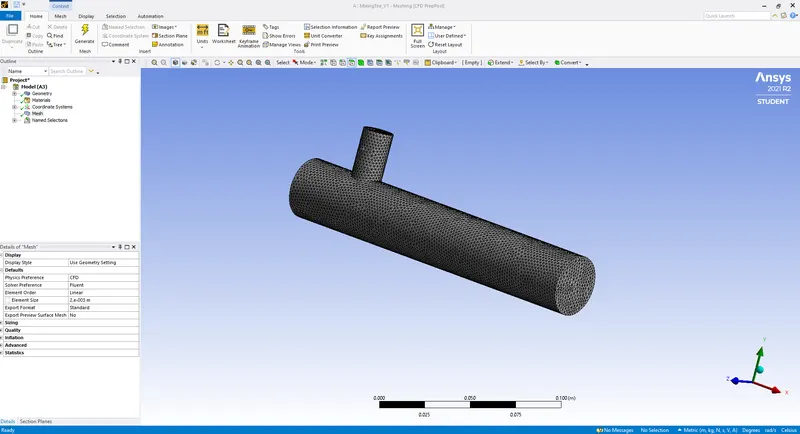
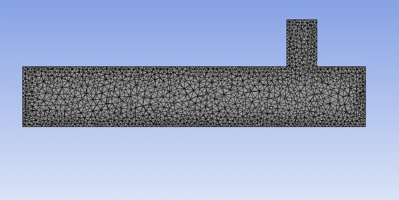
Once the domain is discretized, we move forward to set up the physics in Ansys Fluent.

Setting up the physics

Once in Ansys Fluent, we check the quality of the mesh first and the units to make them conform with that of the mesh. Then the physics (boundary conditions, temperatures, velocity, etc) are set up as stated in the problem description section above.

The gauge pressure is left by default at zero and the temperature by default is 26.78°C.

After the physics are set up, we have defined two reports which will let us compute the average temperature at the outlet.

Results:

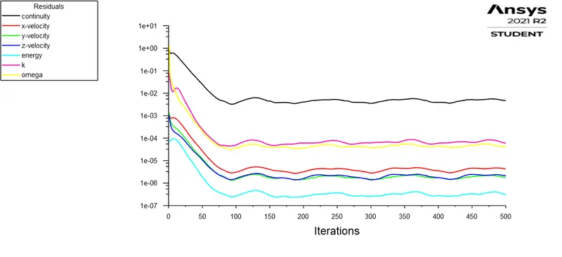
• Residuals from k-ꙍ SST model

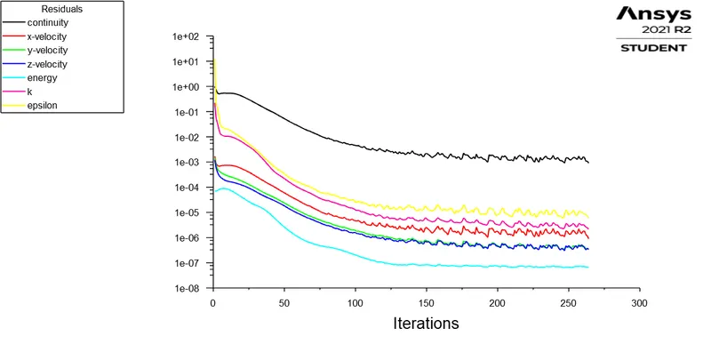
• Residuals from k-Ꜫ model

To run the base testcase, the short mixing tee geometry was chosen with a momentum ratio equal to 2. By analysing the results from k-ꙍ SST and k-Ꜫ turbulence models, the k-ꙍ SST model is chosen for further testcases. This choice is supported by the fact that the results from that model are much closer to the analytical results from the formula given below:

`T_mixture=(m_hot*T_hot+m_cold*T_cold)/(m_hot+m_cold )`

`T_mixture=(m_hot*h_hot+m_cold*h_cold)/(m_hot+m_cold )`

Using the above formula, the mixture temperature Considering the momentum ratio=4 is obtained as follows:

Area (hot inlet)	Area (cold inlet)	Mass flow rate (hot inlet)	Mass flow rate (cold inlet)	Velocity (Hot inlet) m/s	Velocity (Cold inlet) m/s	T_hot (°C)	T_cold (°C)	T_mixture (°C)
0.000956	0.000253	0.003512	0.003724	3	12	36	19	27.25

• Grid independence test

To carry out this test, three different grid sizes are used and the geometry used is the short mixing tee at momentum ratio=4.

Results are as follows:

Size	1.2mm	1.5mm	2mm
Outlet Temperature (°C)	27.554	27.568	27.560
% Error	1.09	1.15	1.14

From this table we can say that our problem is independent of the mesh size.

For further cases, the mesh size of 2mm is used

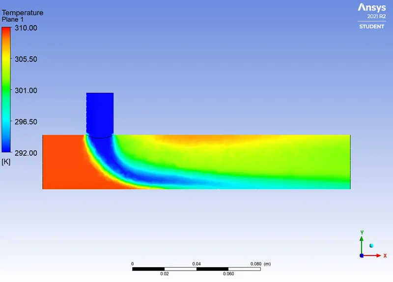
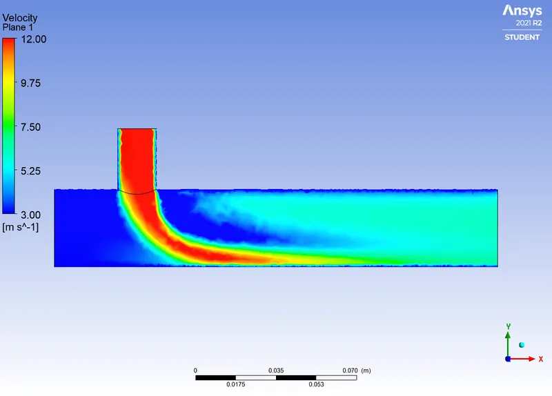
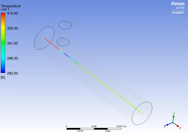
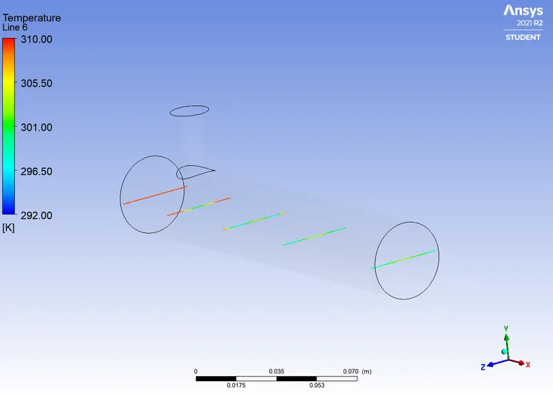
Case1: (Geometry used: short mixing tee)

• Momentum ratio=2

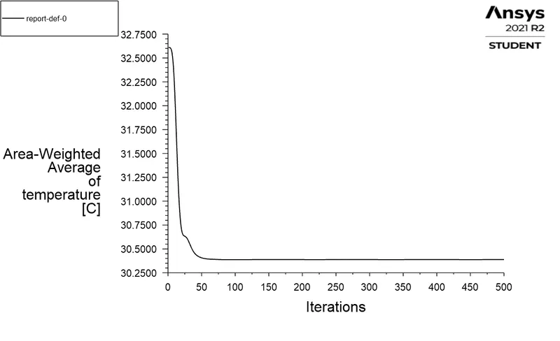
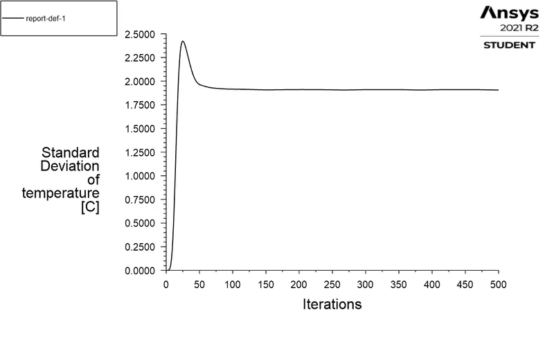
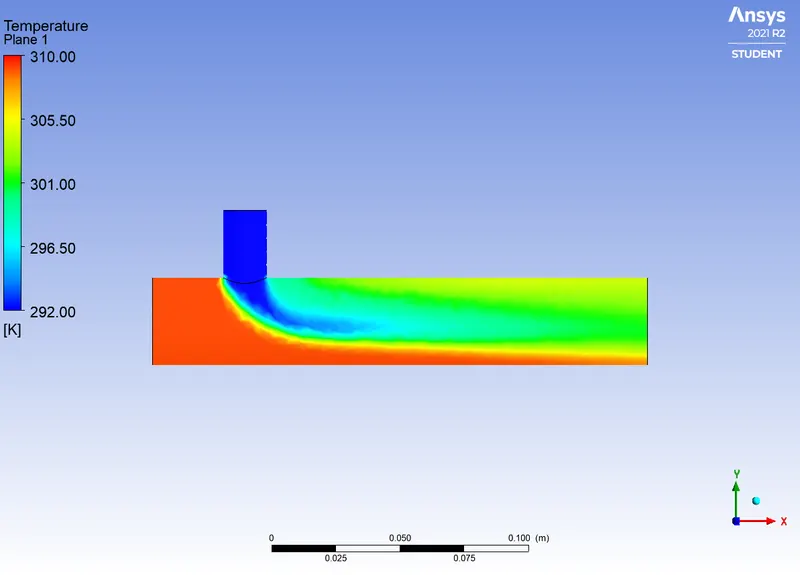
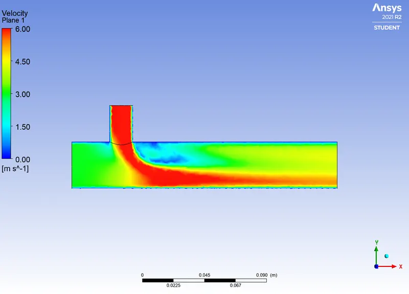
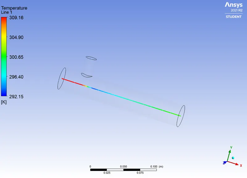
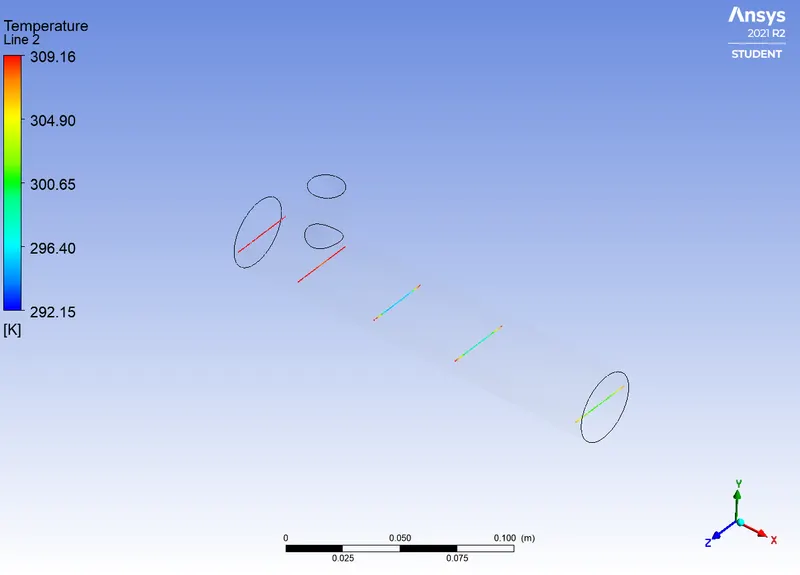
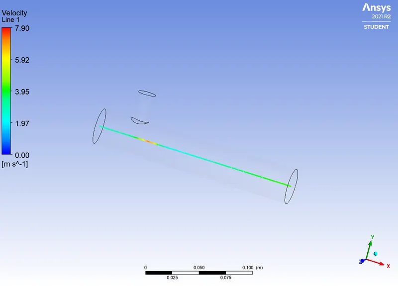
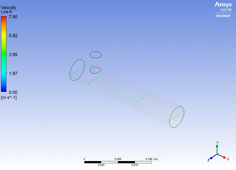
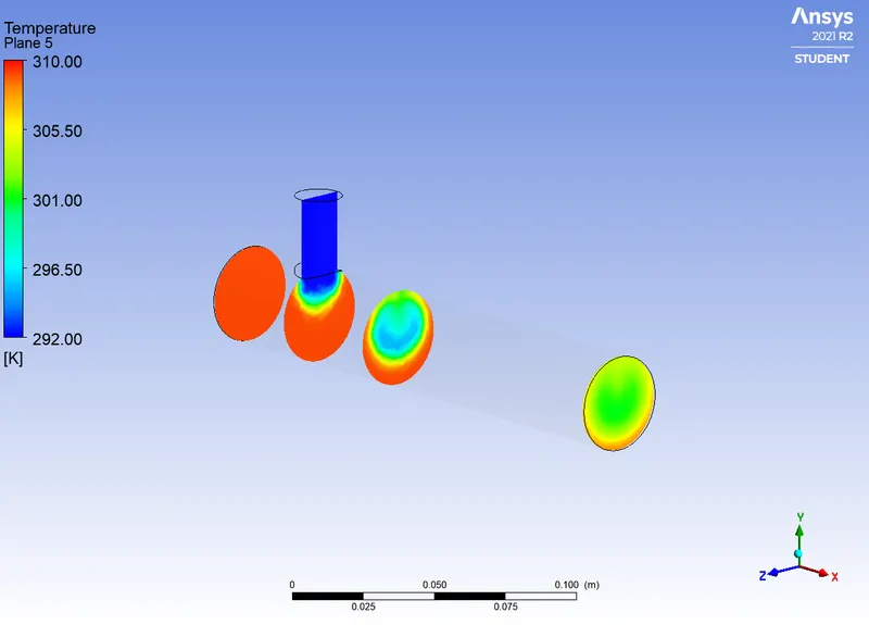
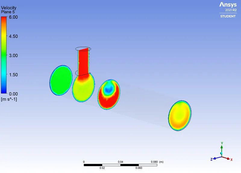
• Momentum ratio=4

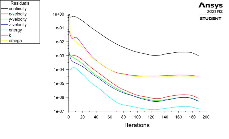
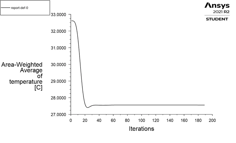
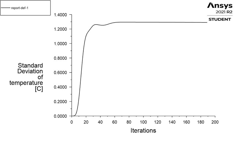
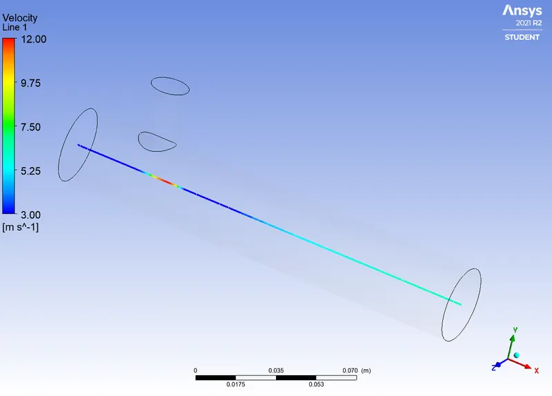
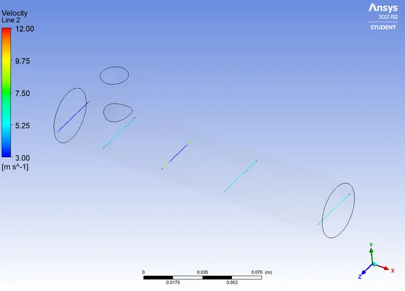
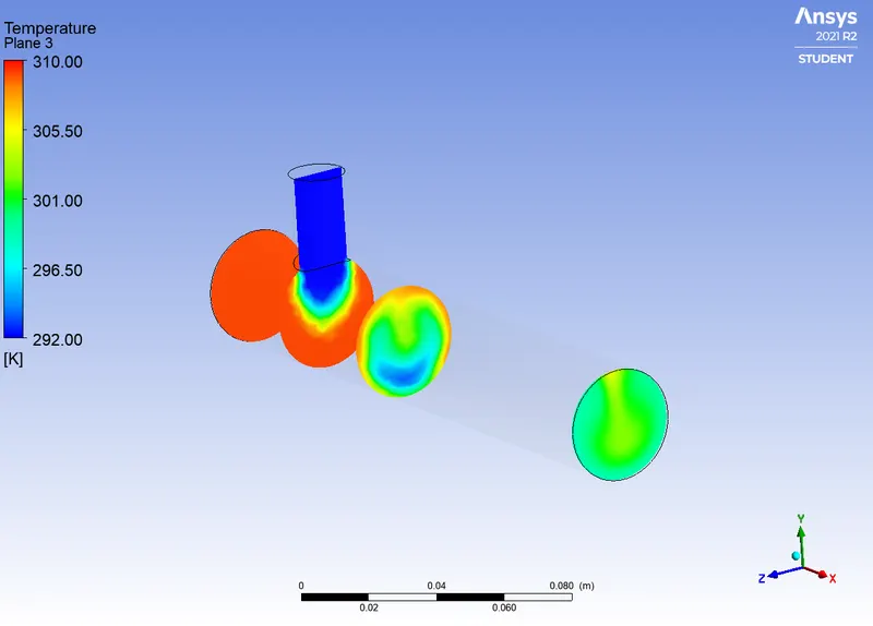
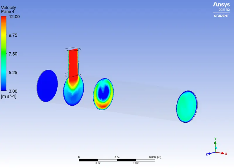
Case2: (Geometry used: long mixing tee)

• Momentum ratio=2

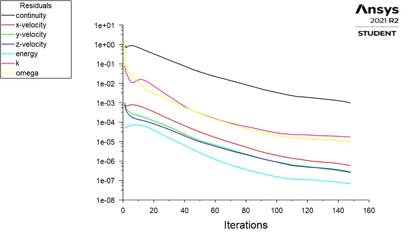
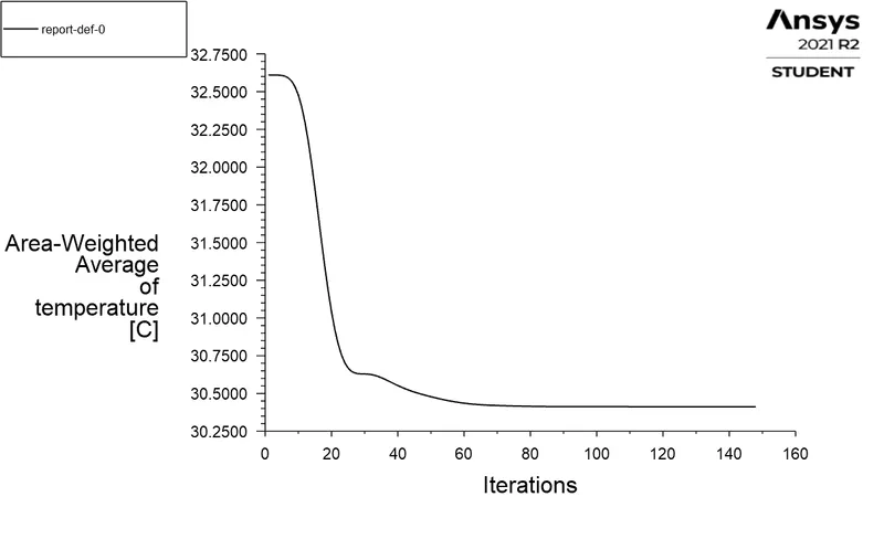
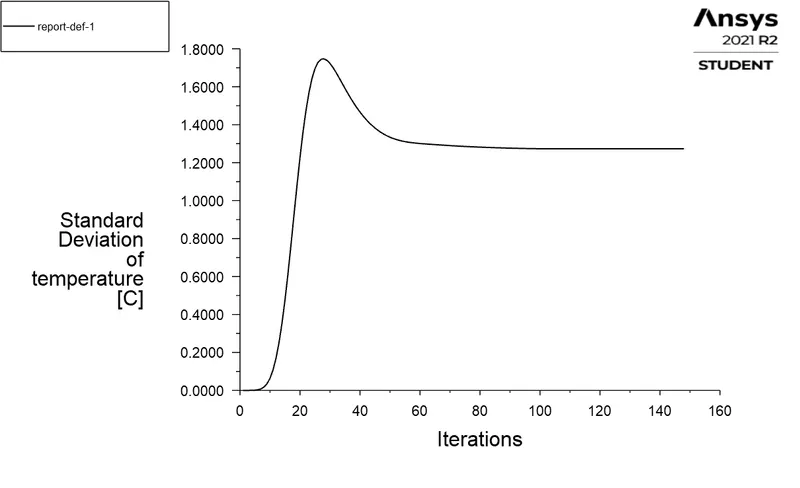
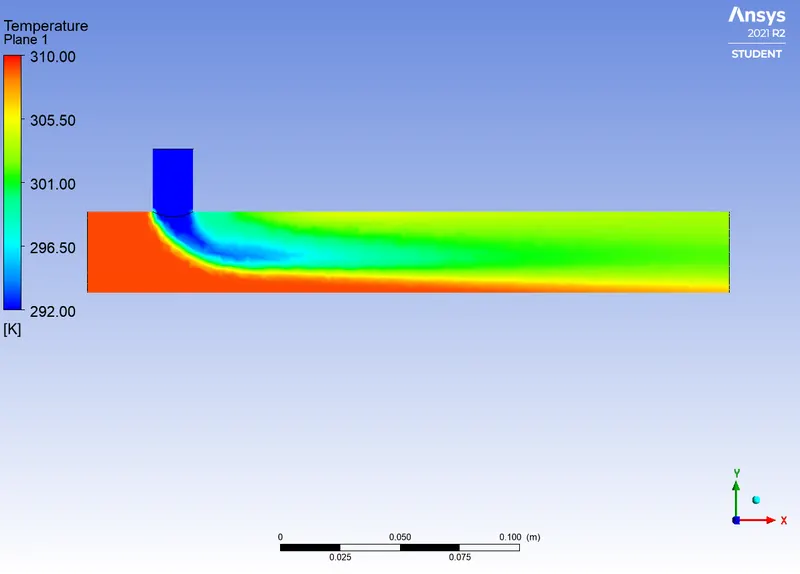
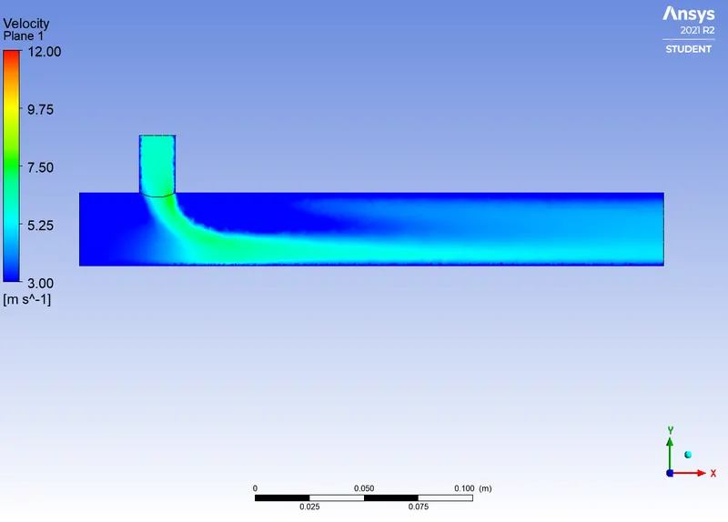
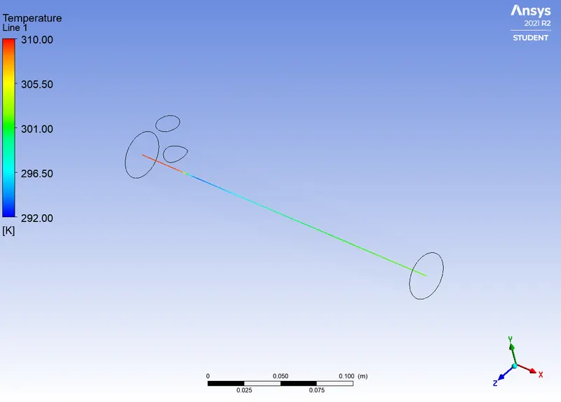
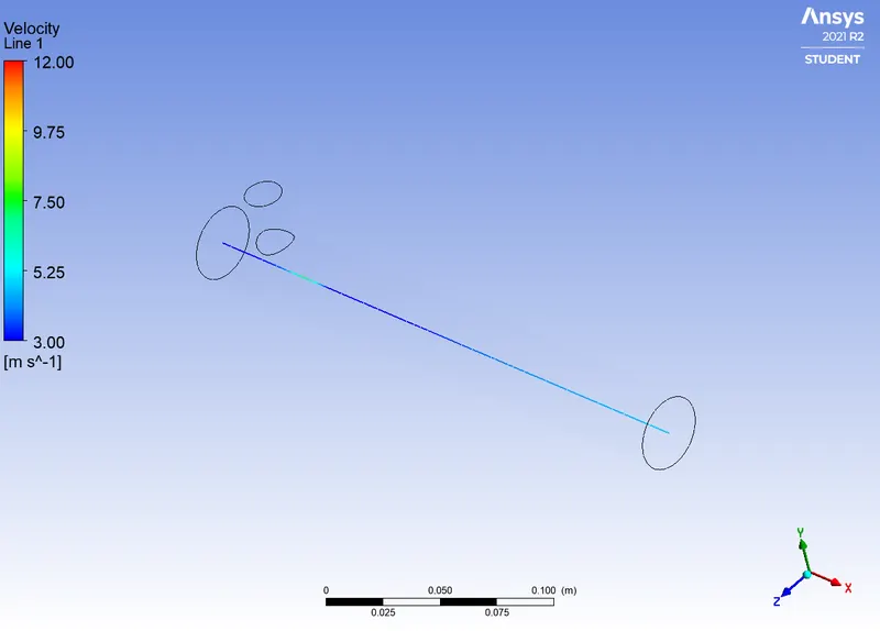
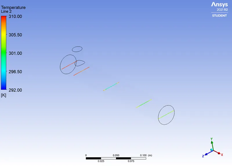
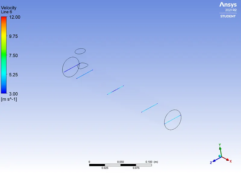
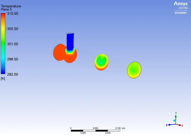
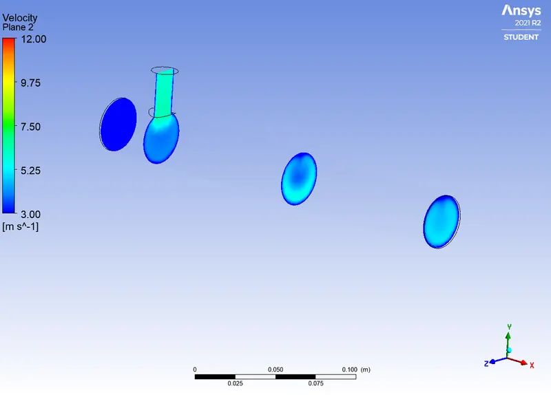
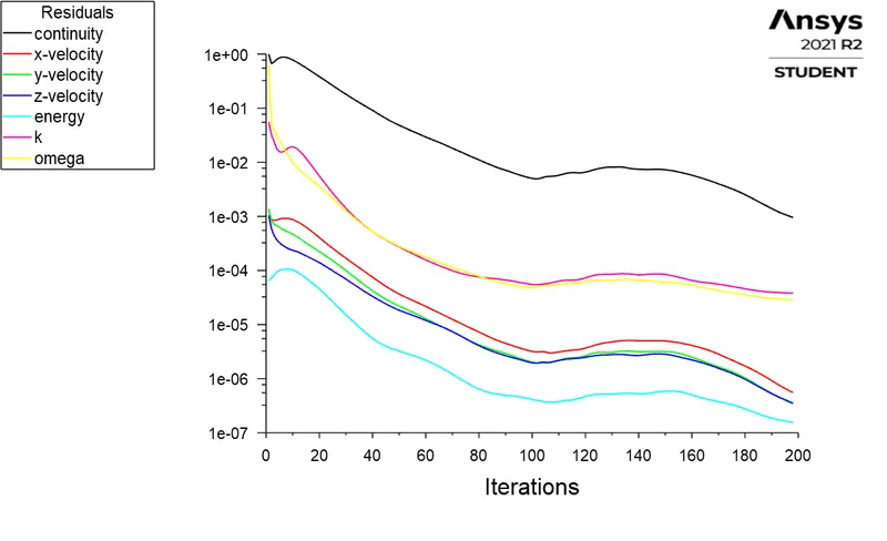
• Momentum ratio=4

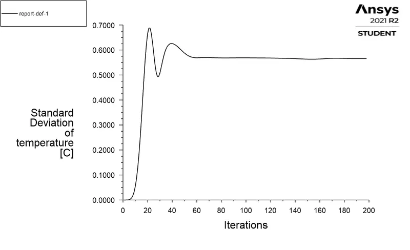
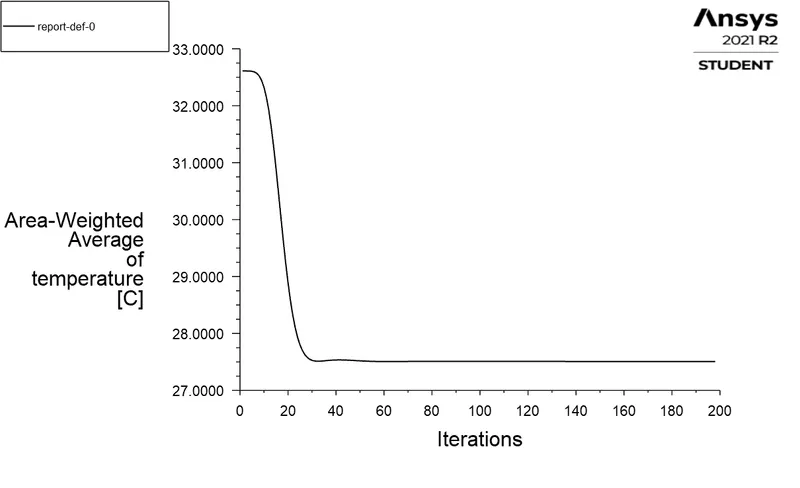
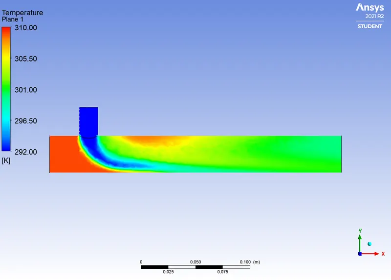
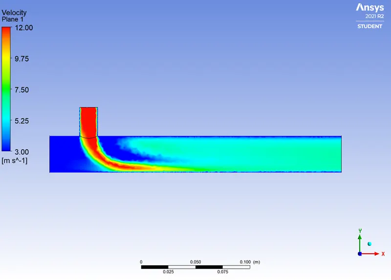
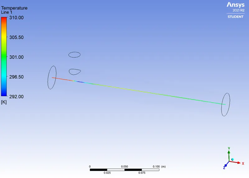
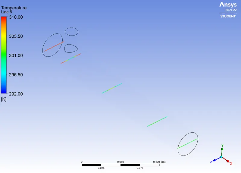
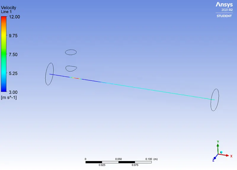
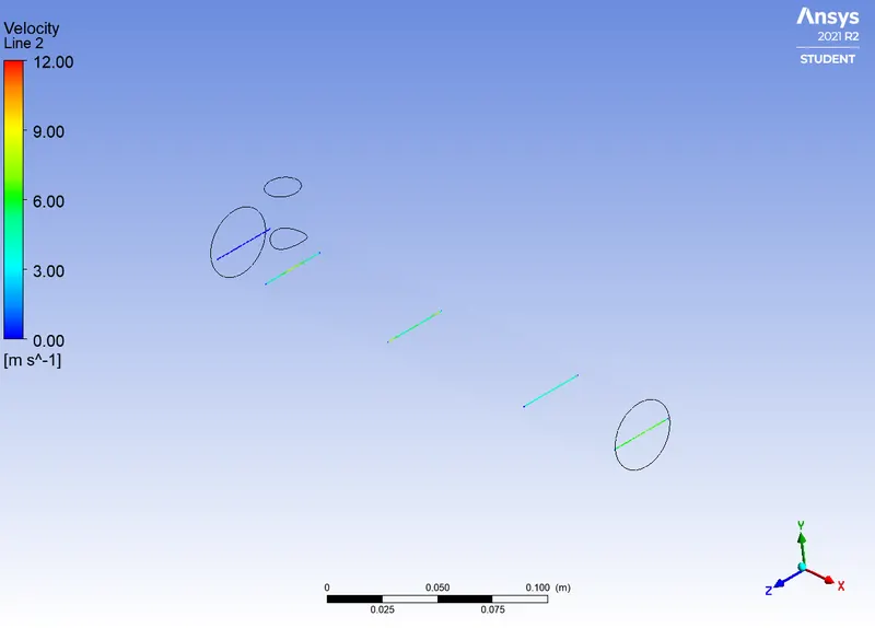
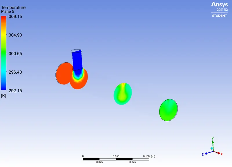
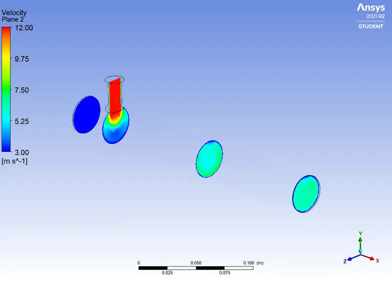
• Comparison of both cases considering

Cell count

Average outlet temperature

Number of iterations for convergence

Cases		Cell count	Average outlet temperature(°C)	Number of iterations for convergence
Case1 (Short geometry)	Momentum Ratio=2	104716	30.39	100
	Momentum Ratio=4	104716	27.56	130
Case2 (Long geometry)	Momentum Ratio=2	138811	30.41	150
	Momentum Ratio=4	138811	27.50	200

Conclusion

To summarize, we have to say from the above results that the outlet temperature drops down significantly in both testcases. This is caused by the higher velocity at the cold inlet. Moreover, slight effect of geometry length is noted on the outlet temperature. Thus, considering the outlet temperature and the standard deviation, we recommend long geometry with high momentum ratio.