CURVE FITTING USING MATLAB

AIM: The aim of this program is to write a MATLAB code to fit a linear and cubic polynomial for the cp data.

It aims to show the split wise method and explain all the parameters involved in the measurement of the fitness characteristics.

OBJECTIVES:

• Know the importance of curve fitting in real life
• Learn how to make a curve fit perfectly
• Learn the difference between best fit and perfect fit and further how to get the best fit
• Learn how to improve a curve fit especially the cubic fit

THEORY:

Curve fitting is the process of constructing a curve, or mathematical function, that has the best fit to a series of data points possibly subject to constraints. Curve fitting can involve either interpolation, where an exact fit to the data is required.

In order to find a curve which satisfies the data under question, there are four quantities which help us measure the goodness of fit criteria or how well the equation is representing the datapoints.

1. The sum of squares due to error (SSE)

`SSE(Sum Of Squared Errors)= ∑_(i=1)^n(Y(i)-f(x(i)))^2`

Where y = f(x) is the fit curve

2. R-square

`R^2=(SSR)/(SST)`

Where

SSR = Sum of squares of the regression which is basically the square of the difference between the value of the fitting function at a given point and the arithmetic mean of the dataset.

And SST = SSR + SSE

3. Adjusted R-square

`R^2adj=[((1-R^2)(n-1))/(n-k-1)]`

Where

n is the number of datapoints

k is the number of independent variables

4. Root mean squared error (RMSE)

`RMSE=√((∑_(i=1)^n(Y(i)-f(x(i)))^2 )/n)=√(SSE/n)RMSE=√((∑_(i=1)^n(Y(i)-f(x(i)))^2 )/n)=√((SSE)/(n))`

where n is the total number of datapoints available.

• PROGRAM AND STEPWISE EXPLANATION

%This program compares the linear curve fit,cubic curve fit to original data
clear all
close all
clc

%Preparing data
cp_data = load('data');
temperature = cp_data(:,1);
cp = cp_data(:,2);



%curve fit
 
%cp = a*T + b
coef_one = polyfit(temperature,cp,1);
Linear_predicted_cp = polyval(coef_one,temperature);
%cp = a*T^3 + b*T^2 + c*T + d

coef_two = polyfit(temperature,cp,3);
Cubic_predicted_cp = polyval(coef_two,temperature);

%Comparing my Linear curve fit with the original data
figure(1)

plot(temperature,cp,'linewidth',3)
hold on
plot(temperature,Linear_predicted_cp,'linewidth',3,'color','r') 
title('Comparing my Linear curve fit with the original data')
xlabel('Temperature [K]');
ylabel('Specific heat [KJ/Kmol-K]')
legend('Original dataset','Linear curve fit')

%Comparing my Cubic curve fit with the original data
figure(2)

plot(temperature,cp,'linewidth',3)
hold on
plot(temperature,Cubic_predicted_cp,'linewidth',3,'color','g')
title('Comparing my Cubic curve fit with the original data')
xlabel('Temperature [K]');
ylabel('Specific heat [KJ/Kmol-K]')
legend('Original dataset','Cubic curve fit')

OUTPUT:

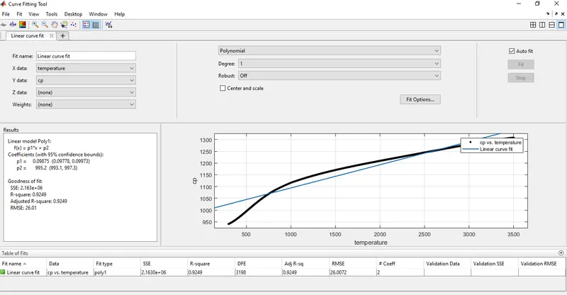
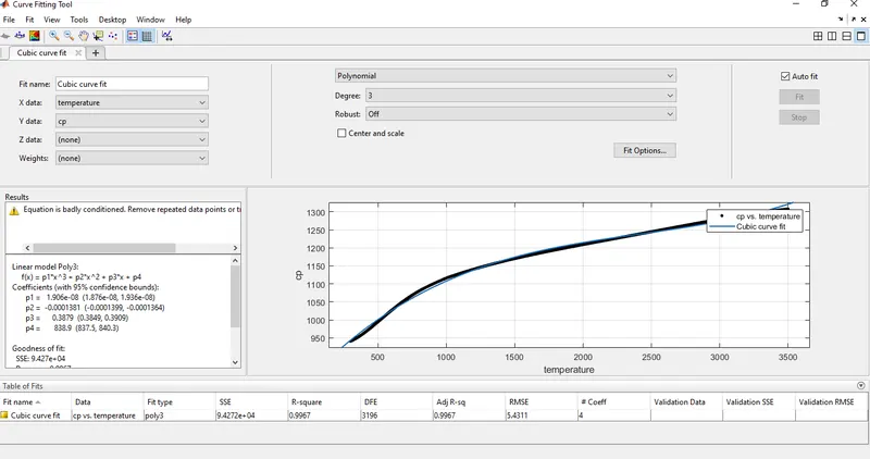
• STEPWISE EXPLANATION

1. Data loading
2. Assigning temperature and specific heat values to temperature and cp variables
3. Calculation of polynomial coefficients using ‘polyfit’ function.
4. Here, we have to find coefficients for linear polynomial and cubic polynomial.

4. At this level we have to predict the values of cp for both linear polynomial and cubic polynomial cases
5. After that we have to plot the graph of temperature versus Specific heat (cp) for each case.
6. Now we have to find the values of the four quantities which help us decide about the goodness of the fit that are SSE, R-square, Adj R-sq, RMSE; and to do so we make use of curve fitting tool box.

PROGRAM TO SHOW THE SPLITWISE METYHOD

%Code to show split wise method
clear all
close all
clc

%Preparing data
cp_data = load('data');
temperature = cp_data(:,1);
cp = cp_data(:,2);
%Separation of data
cp_1 = cp([1:1600]);
temperature_1 = temperature([1:1600]);
cp_2 = cp([1601:3200]);
temperature_2 = temperature([1601:3200]);

figure(1)
%Plotting temperature vs cp using original data
plot(temperature,cp,'linewidth',3,'color','b')
hold on

%Predicting cp values for multiple datasets using fit function for the
%first half
 [Linear_predicted_cp_1,Linear_GOF_1] = fit(temperature_1,cp_1,'poly1')  %Linear_GOF_1 is the godness of fit for first half using polynome of degre one
 plot(Linear_predicted_cp_1,'r')

 %Predicting cp values for multiple datasets using fit function for the
%second half
[Linear_predicted_cp_2,Linear_GOF_2] = fit(temperature_1,cp_2,'poly1')%Linear_GOF_2 is the godness of fit for second half using polynome of degre one 
 plot(Linear_predicted_cp_2,'g')
 hold off

 title('Splitwise method using polynomial of degre 1')
 xlabel('Temperature [K]')
 ylabel('Specific Heat [KJ/Kmol-K]')
 legend('original data', 'dataset_1 Temp[1-1600]','dataset_2 Temp[1601-3200]')
 
figure(2)
%Plotting temperature vs cp using original data
plot(temperature,cp,'linewidth',3,'color','b')
hold on

%Predicting cp values for multiple datasets using fit function for the
%first half
 [Cubic_predicted_cp_1,Cubic_GOF_1] = fit(temperature_1,cp_1,'poly3')  %Cubic_GOF_1 is the godness of fit for first half using polynomial of degre 3
 plot(Cubic_predicted_cp_1,'r')

 %Predicting cp values for multiple datasets using fit function for the
%second half
[Cubic_predicted_cp_2,Cubic_GOF_2] = fit(temperature_1,cp_2,'poly3')%Cubic_GOF_2 is the godness of fit for second half using polynomial of degre 3
 plot(Cubic_predicted_cp_2,'g')
 hold off

 title('Splitwise method using polynomial of degre 3')
 xlabel('Temperature [K]')
 ylabel('Specific Heat [KJ/Kmol-K]')
 legend('original data', 'data set_1  Temp[1-1600]','data set_2 Temp[1601-3200]')

OUTPUT:

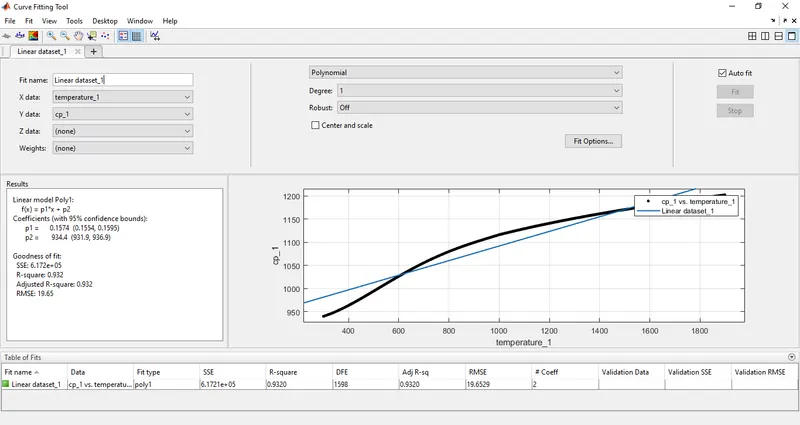
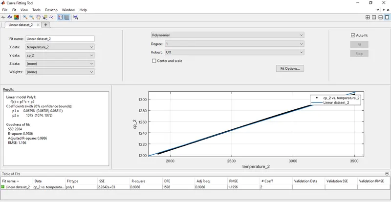
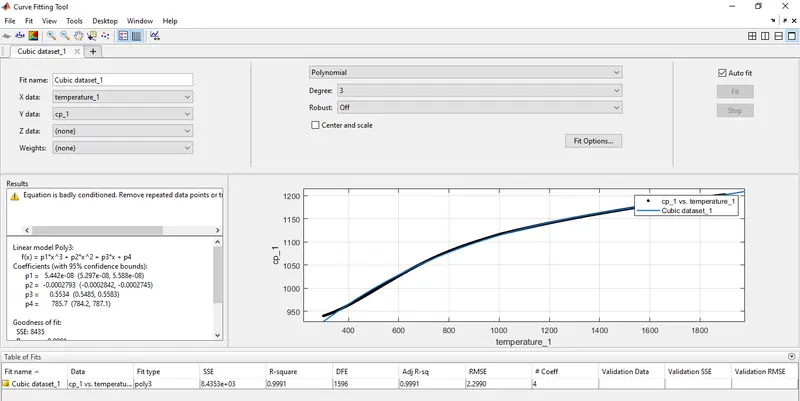
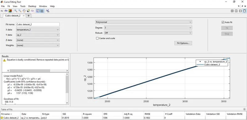
As it can be seen through the images, the last one is depicting the second half dataset with polynomial of degre 3. And in that case, the R-Square is equal to 1. This means that the curve fit could be perfect in this case but there is a message in the result tab saying that the equation is badly conditioned.

So to overcome this we have to check center and scale box.

Furthermore,these four images above can be visualized on the following two images:

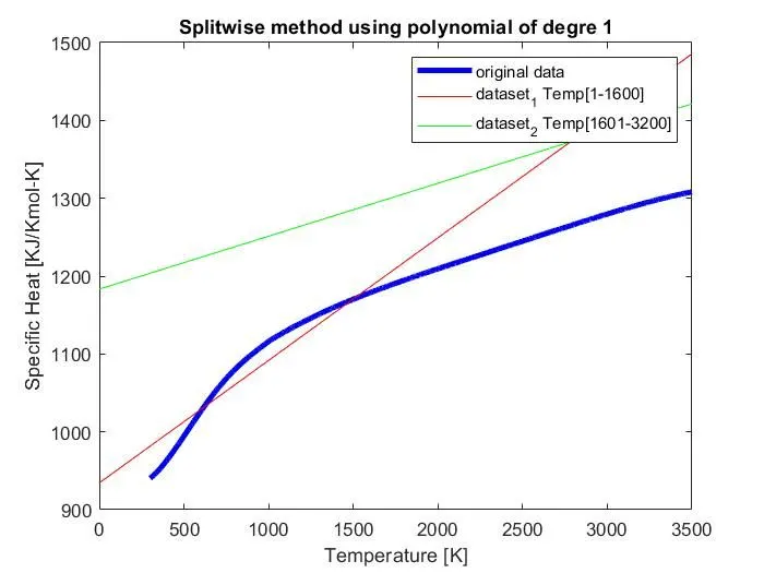
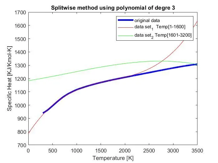
Considering all the above curve fits, we have to notice that as we increase the degre of the polynomial, the error between the curve fit and the original data is reduced and by using splitwise method, the goodness of the curve fit is improved.

Questions/Answers

How to make a curve fit perfectly ?

In order to get a perfect fit, we have to interpolate the datasets which means that we have to divide the original data into multiple datasets by considering the errors and using center and scale option if necessary.

How to get the best fit ?

Through our work, we can say that in order for one to get the best fit,we have the possibility to use splitwise method, or increase the order of the polynomial or to use the four parameters mentioned above in the the theory part.

What could be done to improve the cubic fit?

Here also, through our work we realised that the cubic curve fit in the case of splitwise method gets improved. Thus we can say that in order to improve the cubic curve fit, we have to use the splitwise method and center and scale option.

REFERENCES:

https://skill-lync.com/projects/Week-4-Curve-fitting-31550#:~:text=How%20to%20make%20perfect%20fit,that%20perticular%20degree%20of%20polynomial.