Simulating Cyclone separator with Discrete Phase Modelling

Aim: To perform analysis on the cyclone separator and calculate the separation efficiency and pressure drop

Objectives

There are multiple objectives behind this work which can be summarized as follows:

• Develop the ability to write a few words about any four empirical models used to calculate the cyclone separator efficiency.
• To perform an analysis on a given cyclone separator model by varying the particle diameter from 1 μm to 5 μm and calculate the separation efficiency in each case.
• To perform an analysis on a given cyclone separator model by varying the particle velocity from 1 m/s to 5 m/s and calculate the separation efficiency and pressure drop in each case.

Introduction

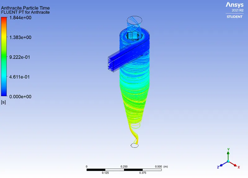
Cyclones are devices widely used in industries to separate dust form gas or for product recovery. These devices employ a centrifugal force generated by a spinning gas stream to separate particles from carrier gas. They are designed to be simple, low capital cost, and almost maintenance-free, making them ideal precleaners before more expensive control devices such as bag-houses or electrostatic precipitators. Cyclones are designed is such a way to withstand high temperature and pressure conditions. Cyclones are used to remove large particles for both air pollution control and process use. For large particles (more than 5 μm), the efficiency of cyclones can reach 99%. They can also be used to remove coal dust from a power plant or used as spray dryer or gasification reactor. In order to evaluate the design and performance of a cyclone, we are interested in the collection efficiency of particles and the pressure drop through the cyclone. Thus, in this work, analysis on the cyclone separator is carried out using Discrete Phase Modelling in Ansys-Fluent. The simulation is done in two parts using structural mesh, RNG k-Ꜫ model with Swirl dominated flow and standard wall function, and “Reflect” boundary condition for inlet and wall; “Escape” boundary condition for the top outlet of the cyclone and “Trap” boundary condition for the bottom outlet. The first part is to perform the analysis by varying the particle diameter from 1 μm to 5 while keeping the flow and particle velocity at 3 m/s. The second part is to perform the simulation varying the velocity from 1 m/s to 5 m/s while keeping the particle diameter at 5 μm and velocity of flow and particle equal. The separation efficiency and pressure drop are calculated and results are discussed.

Theory

Nowadays, CFD has a great potential to predict the flow field characteristics and particle trajectories. The analysis of the swirling turbulent flow in a cyclone is complicated process which requires sophisticated numerical methods in CFD. These techniques are developed based on empirical models which are as follows: Iozia and Leith, Koch and Licht, Li and Wang, and Lapple models.

• Iozia and Leith model

Iozia and Leith logistic model is a modified version of Barth model, which is developed based on force balance. The model assumes that a particle carried by the vortex endures the influence of two forces: a centrifugal force Z and a flow resistance W. The collection efficiency ηi of a particle diameter `d_pi` can be calculated from `η_i=1/(1+(d_pc/d_pi)^β )` `β` is an expression for slope parameter derived based on the statistical analysis of experiment al data of a cyclone with D=0.25m given as `β=0.62-0.87 ln⁡((d_pc)/100)+5.21 ln⁡((ab)/D^2 )+1.05[ln⁡((ab)/D^2 )]^2`

• Li and Wang model

This model includes particle bounce or re-entrainment and turbulent diffusion at the cyclone wall. A two-dimensional analytical expression of particle distribution in the cyclone is obtained. Li and Wang model was developed based on the following assumptions:

-The radial particle velocity and the radial concentration profile are not constant for uncollected particles within the cyclone.

-Boundary conditions with the consideration of turbulent diffusion coefficient and particle bounce re-entrainment on the cyclone wall are:

`c=c_o,` at `θ=0`

`D_r (∂c)/(∂r)=(1-α)ωc,` at `r=D/2`

-The tangential velocity is related to the radius of cyclone by:

`uR^n=constant`

The concentration distribution in a cyclone is given as:

`c(r,θ)=(c_0 (r_ω-r_n ) e^{-λ[1/K(1+n) r^(1+n) ]} )/(∫_(r_n)^(r_ω)e^{1/K(1+n) r^(1+n) }dr )` where `K=((1-n)(ρ_p-ρ_g ) d^2 Q)/(18μb(r_ω^(1-n)-r_n^(1-n) ))`

And `λ=((1-α)Kω_ω)/(D_r r_ω^n )` The resultant expression of the collection efficiency for particle of any size is given as `η_i=1-e^(-λθ_1 )`

Where `θ_1=(2π(S+L))/a`

• Koch and Licht model

Koch and Licht collection theory recognized the inherently turbulent nature of cyclones and the distribution of gas residence times within the cyclone. Koch and Licht described particle motion in the entry and collection regions with the additional following assumptions:
• The tangential velocity of a particle is equal to the tangential velocity of the gas flow, i.e., there is no slip in the tangential direction between the particle and the gas.
• The tangential velocity is related to the radius of cyclone by:

`uR^n=constant`

A force balance and an equation on the particles collection yields the grade efficiency ηi.

`η_i=1-e^{-2[(Gτ_i Q)/D^3 (n+1)]^(0.5/((n+1) )) }` Where `G=(8K_c)/(K_a^2 K_b^2 )` `n=1-{1-(12D)^0.14/2.5} {(T+4600)/530}^0.3` ;

`τ_i=(ρ_p d^2_pi)/(18μ)`

G is a factor related to the configuration of the cyclone, n is related to the vortex and is the relaxation term.

• Lapple model

This model was developed based on force balance without considering the flow resistance. Lapple assumed that a particle entering the cyclone is evenly distributed across the inlet opening. The particle that travels from inlet half width to the wall in the cyclone is collected with 50% efficiency. This semi-empirical relationship developed by Lapple to calculate a 50% cut diameter, `d_pc` is `d_pc=[(9μb)/(2πN_e v_i (ρ_p-ρ_g ))]^(1/2)`

Where Ne is the number of revolutions and `N_e=1/a [h+(H-h)/2]`

• Modelling and Pre-processing

Geometry preparation

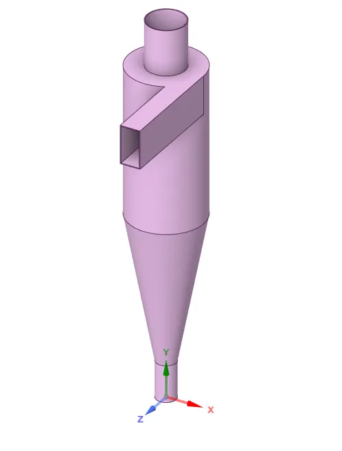
The CAD model is imported in SpaceClaim. Since the analysis is going to be carried out on the fluid volume, the latter is extracted from the CAD model using ‘volume extract’ command under ‘prepare’ option in SpaceClaim. After that, the primitive model/Geometry is suppressed from the physics.

Meshing

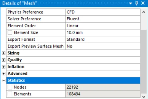
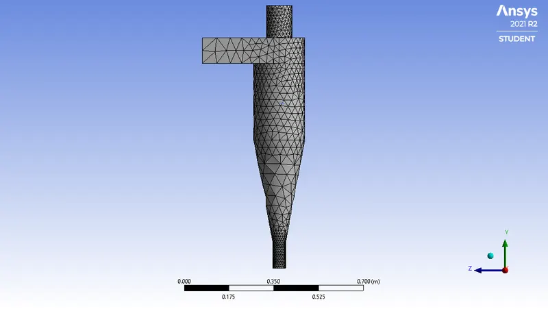
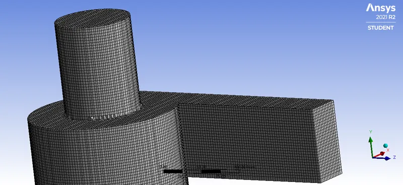
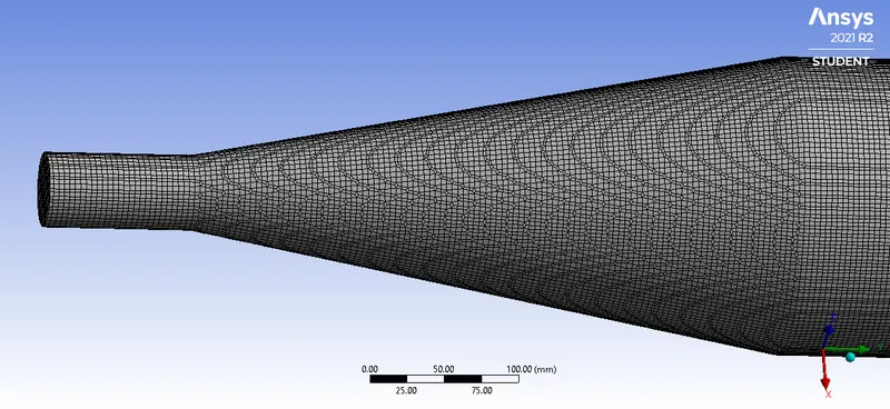
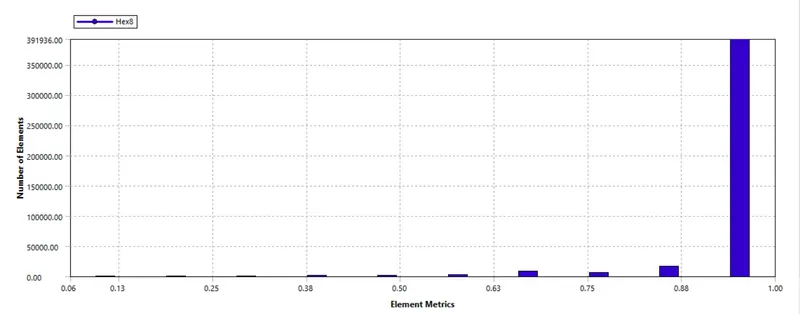
After creating the fluid volume, the model is transferred to the meshing module. The mesh is generated with a default size of 55.916 mm. Then the name selection is done by assigning a characteristic name to corresponding zones. Thus, the inlet, outlet 1 and outlet 2 are defined for the model.

• Mesh Refinement with the use of Cartesian method

Setting up the Case

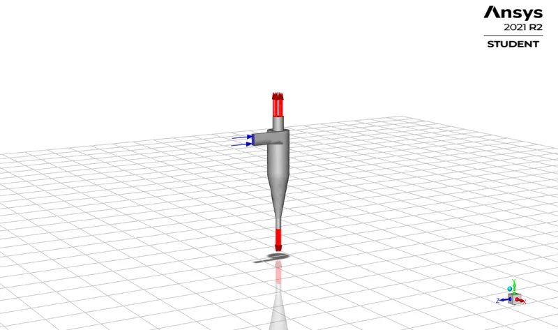
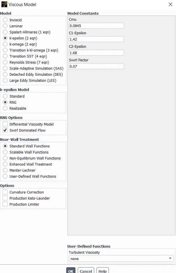
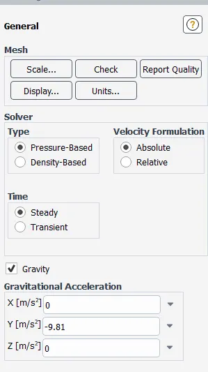
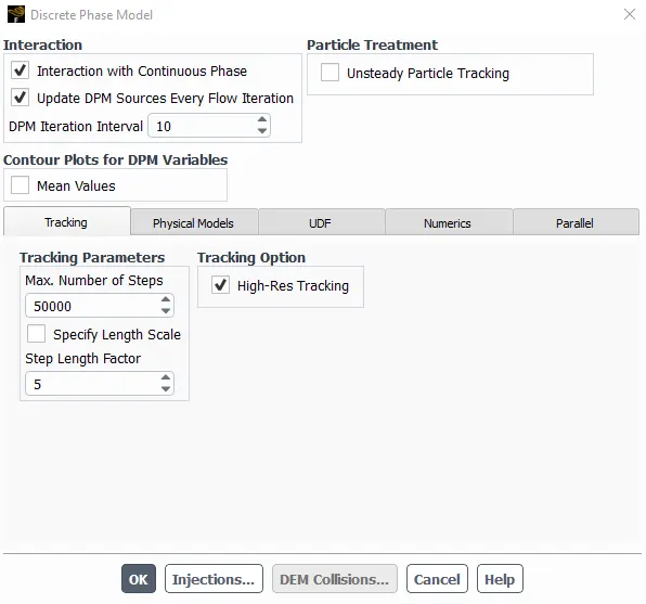
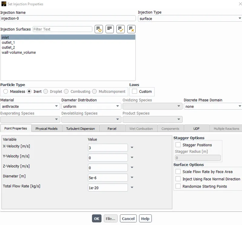
The model is then moved to Fluent for case setting up. Here the steady-state simulation is chosen with gravity enabled is negative y-direction. Under the models, the RNG k-Ꜫ model with Swirl dominated flow and standard wall function is used. The discrete phase model is turned on. The interaction with the continuous phase is enabled in order to use the coupled flow. This is done because the size of the particles injected in the cyclone is very small and the choice between coupled and uncoupled flow is of great interest. The DPM sources are updated at every iteration in order to calculate the corresponding source term at each iteration. The racking parameters are left by default. After that the injection is created where the particles type is inert, the injection type is set to ‘surface’ and the material is anthracite. The particles diameter is set to 5 micrometres and the velocity is set to 3m/s in x-direction.

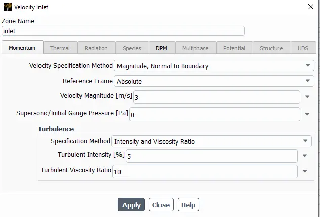
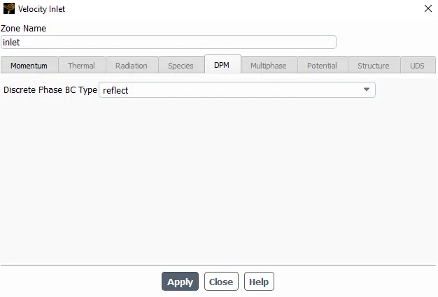
After that, the boundary conditions are defined. For the inlet, the velocity is again set to 3m/s and the Discrete Phase BC type is set to ‘reflect’.

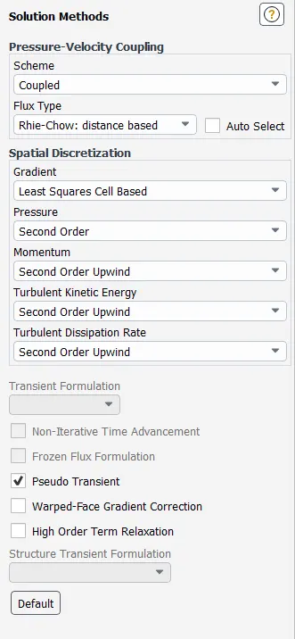
Under the solution method, the Second Order Upwind is used for turbulent kinetic energy and turbulent dissipation rate. This is done since the Second Order Upwind is the most accurate special discretization scheme for this kind of problem.

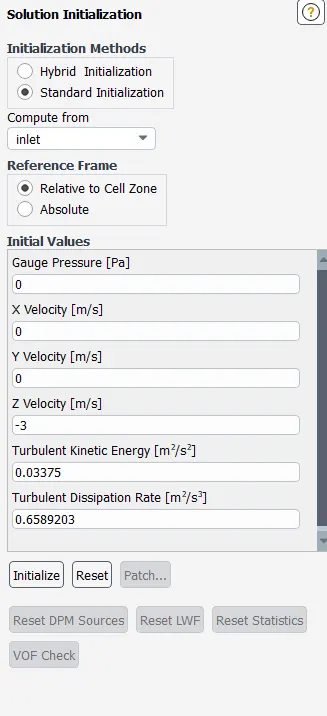
After choosing the standard initialization, the case is computed from the inlet.

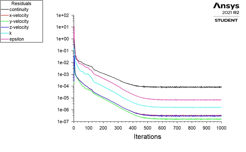
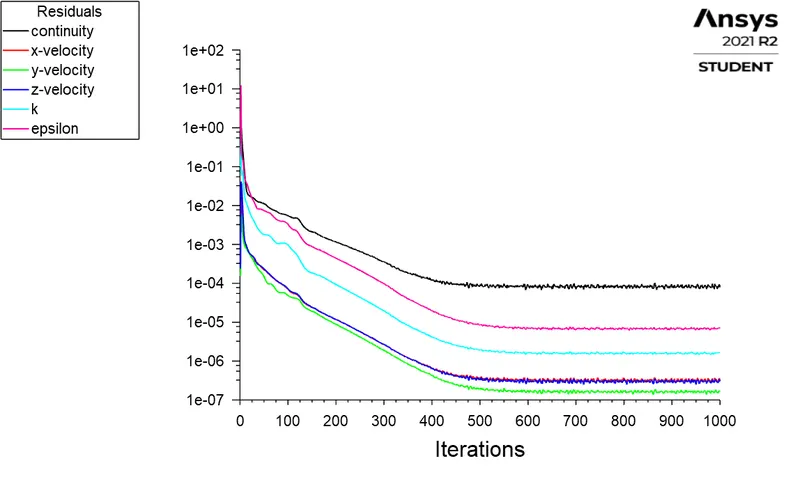
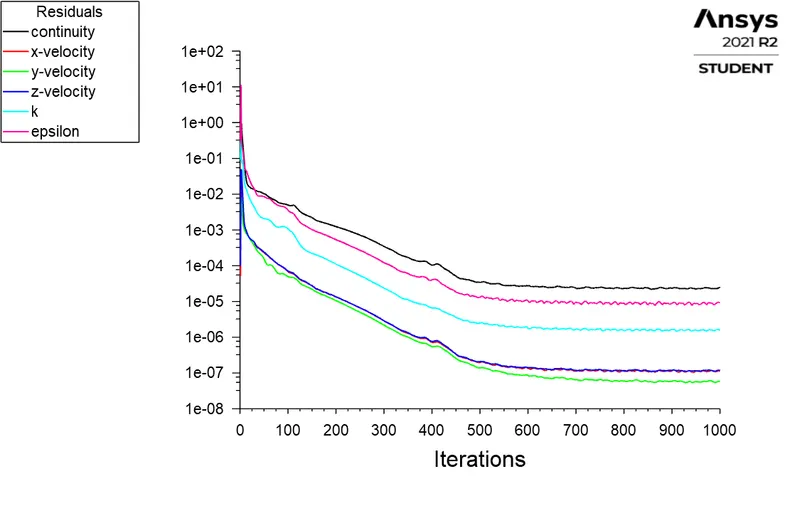
The simulation run for 600 iterations.

Results for the base case

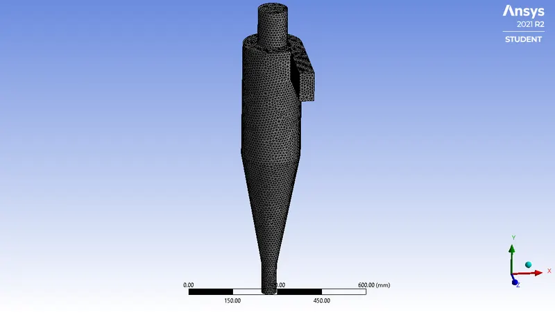
The first remarque is that the number of tracked particles is 4 and the number of escaped particles is 4. This number is too low so we have to work to improve these results. So, to increase the number of tracked particles, a Mesh Refinement is done bringing the mesh size to 10mm. By doing so, the number of tracked particles is increased to 124 and the number of escaped particles is also 124.

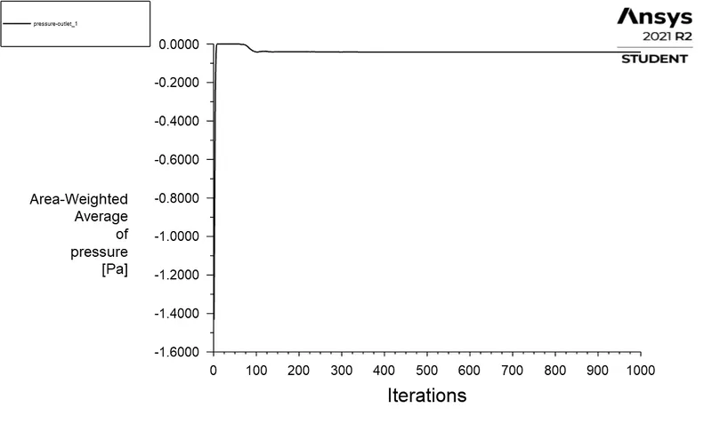
The mass flow on the inlet is then calculated and is found to be equal to 0.018375 [kg s^-1]. At the outlet_1 Mass flow is = -0.0146013 [kg s^-1] and on the outlet_2 the mass Flow is = -0.00377138 [kg s^-1].

Base Case Animation

Results and Discussion

`Separation _efficiency=frac{Number of Particl_es Trapped}{Number of Particl_es Tracked}`

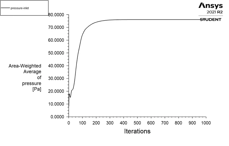
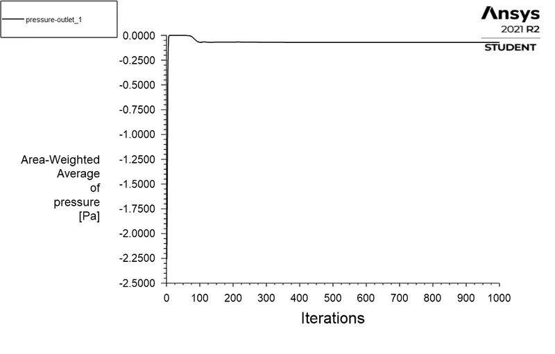
`Pressure Drop=Total Inl_et pressure-Total outl_et pressure`

• Part 1 (Constant velocity=3m/s with varying particle diameter)

• Case1 (Particle size=1μm)

Part1 Case 1 animation

• Case2(Particle size=2μm)

Part1 Case 2 animation

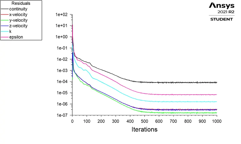
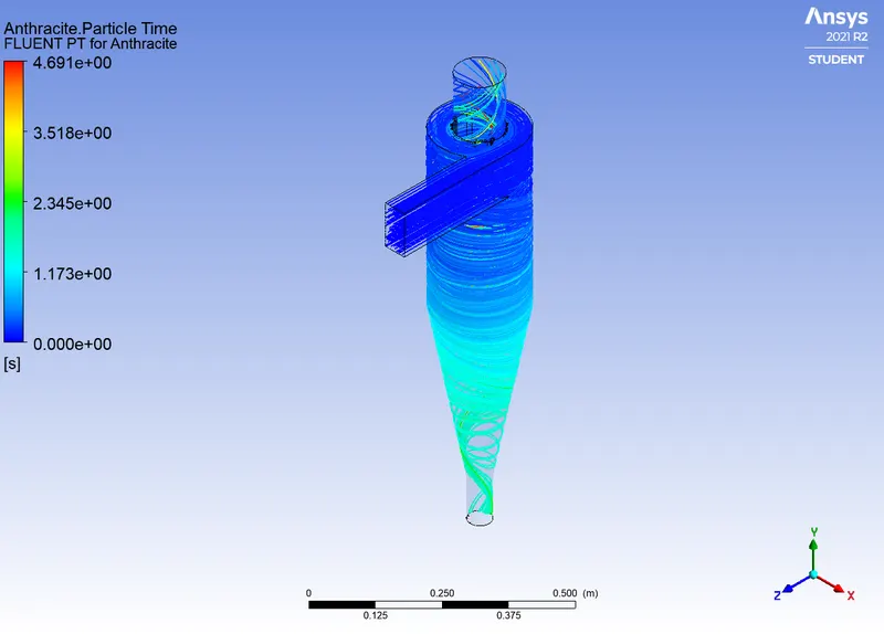
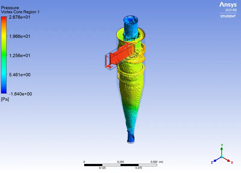
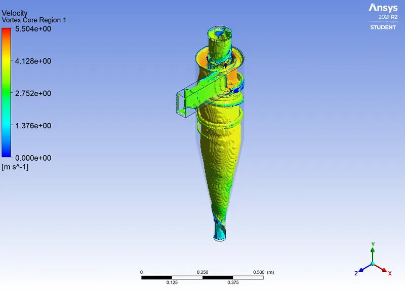
• Case3(Particle size=3μm)

Part1 Case3 Animation

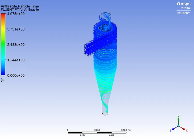
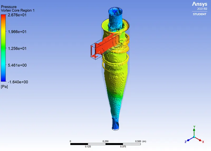
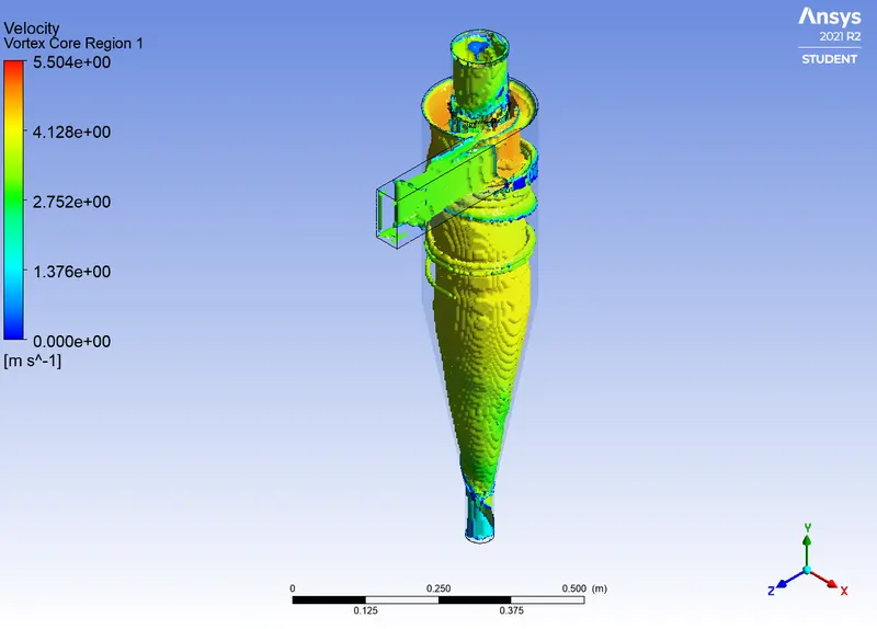
• Case4(Particle size=4μm)

Part1 Case4 Animation

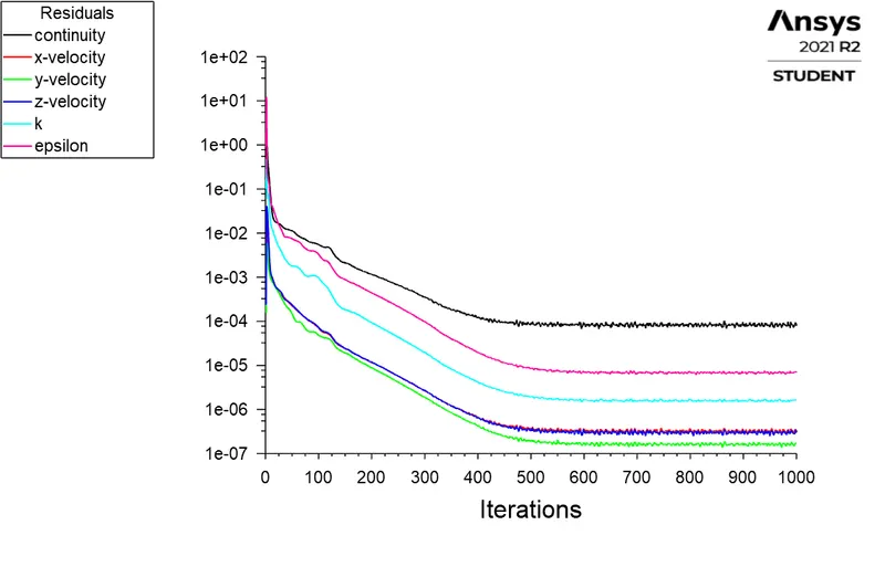
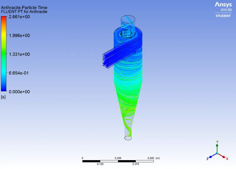
• Case5(Particle size=5μm)

Part 1 Case 5 Animation

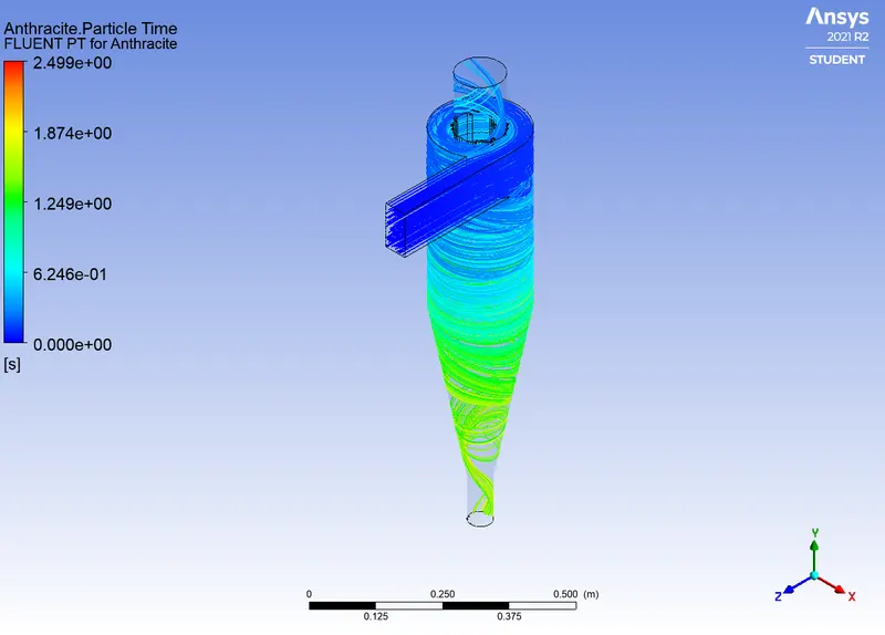
• Part 2 ( The particle diameter is kept at 5μm with a varying velocity)

• Case 1 (Velocity = 1m/s)

Part 2 Case 1 Animation

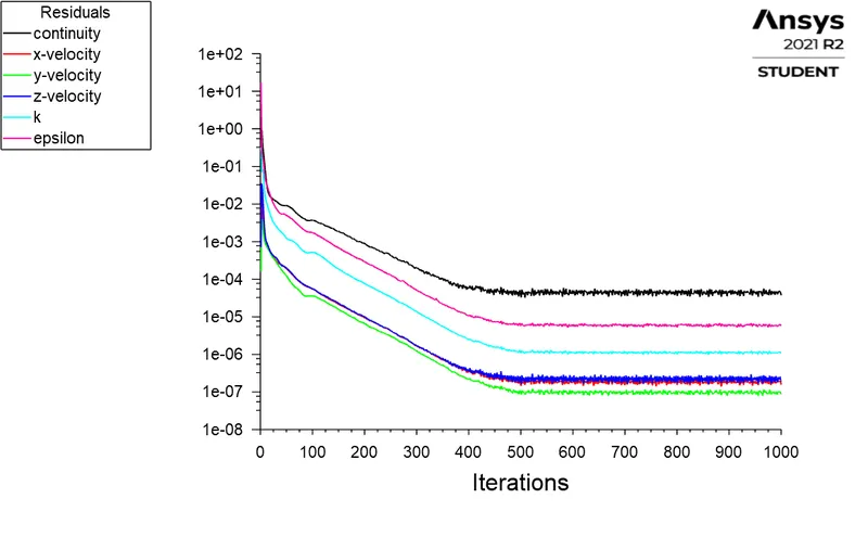
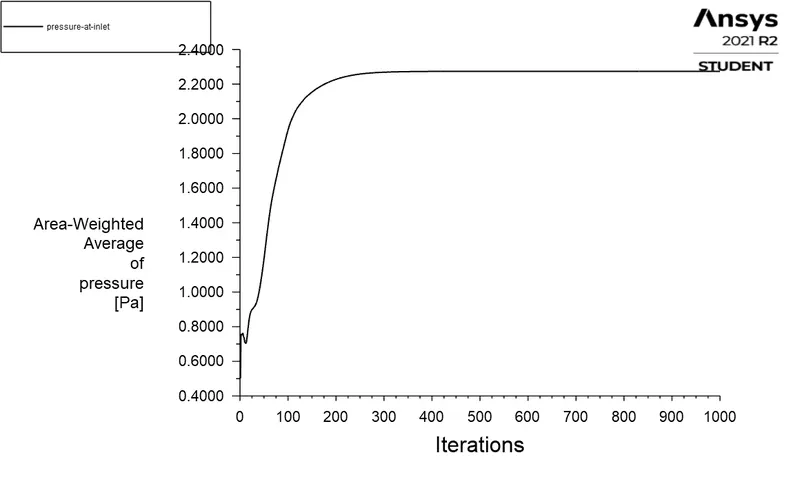
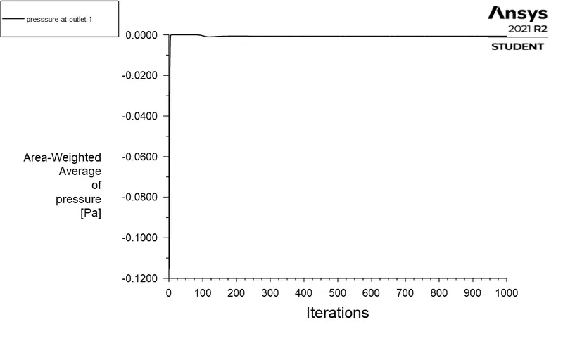
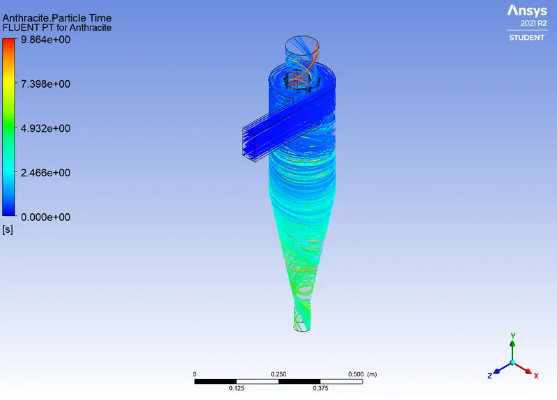
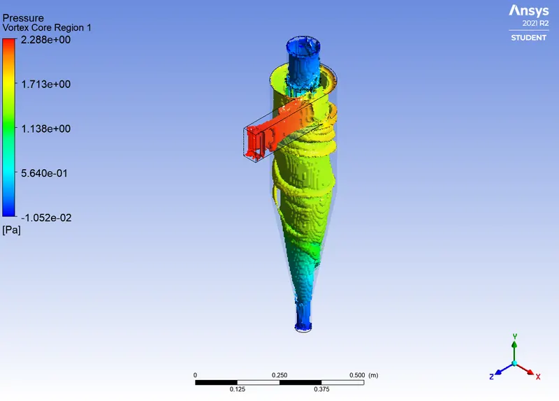
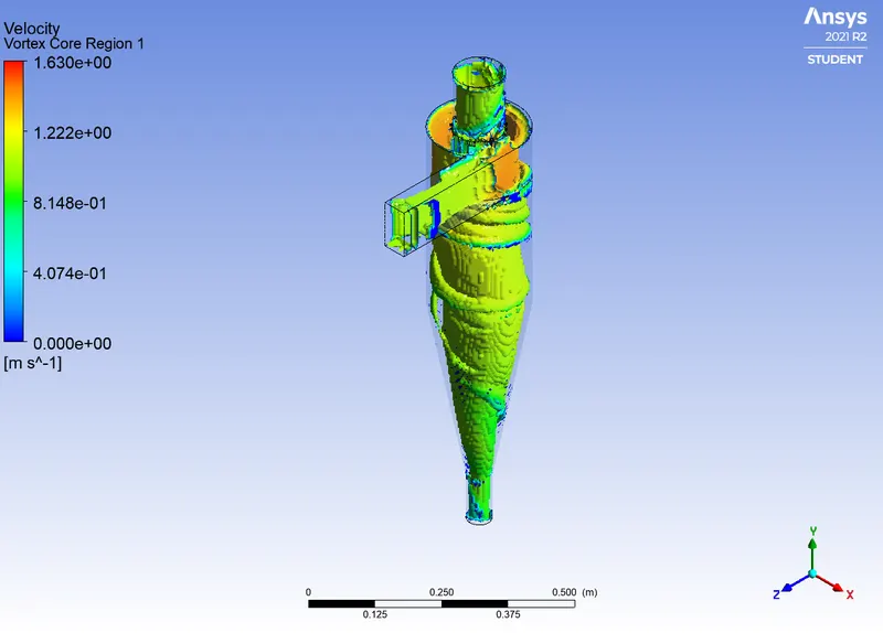
• Case 2 (Velocity = 2m/s)

Part 2 Case2 Animation

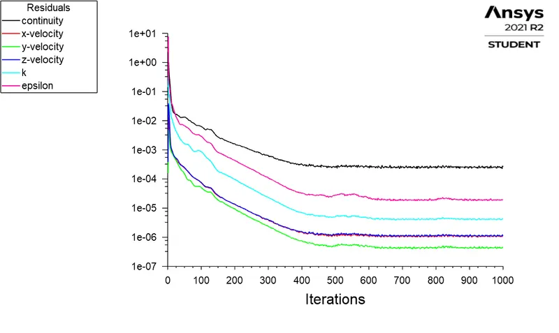
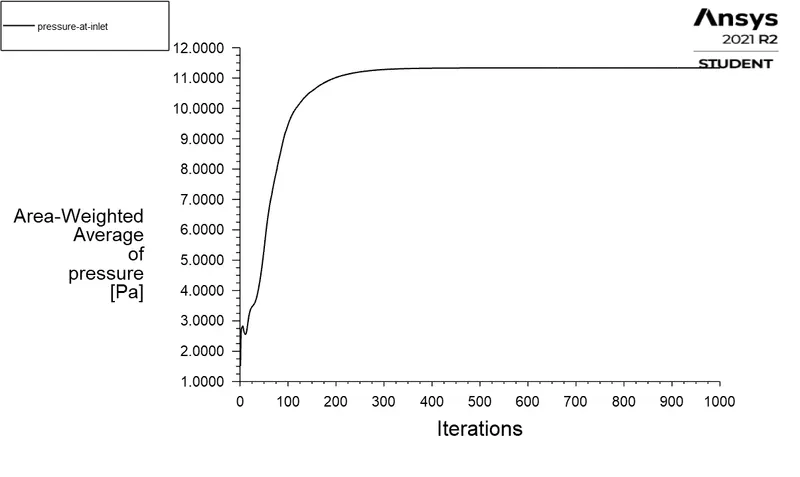
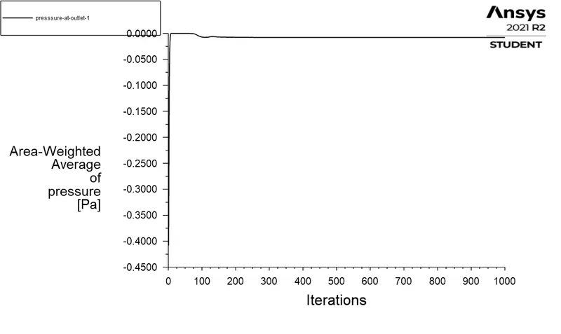
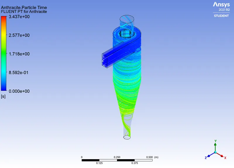
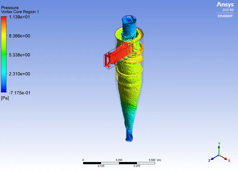
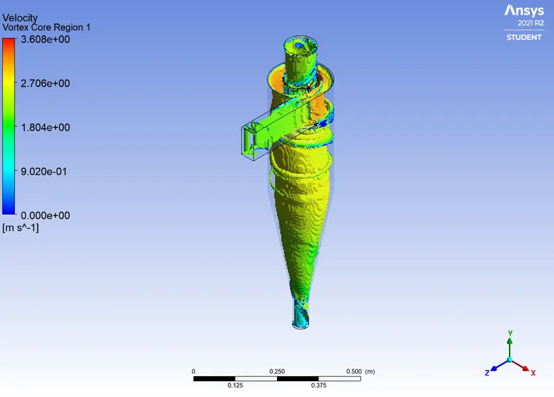
• Case 3 (Velocity = 3m/s)

Part 2 Case 3 Animation

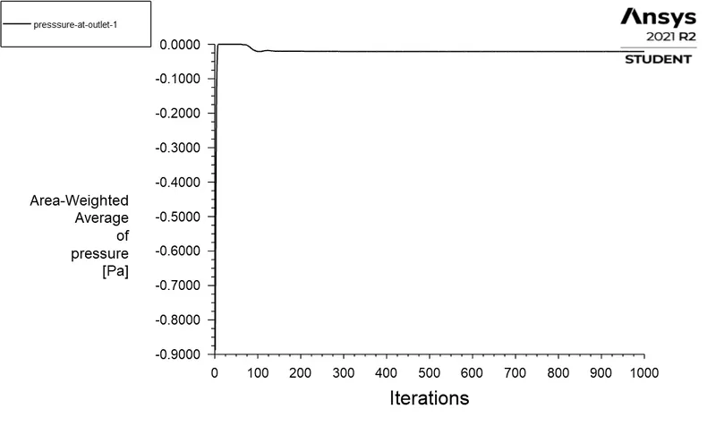
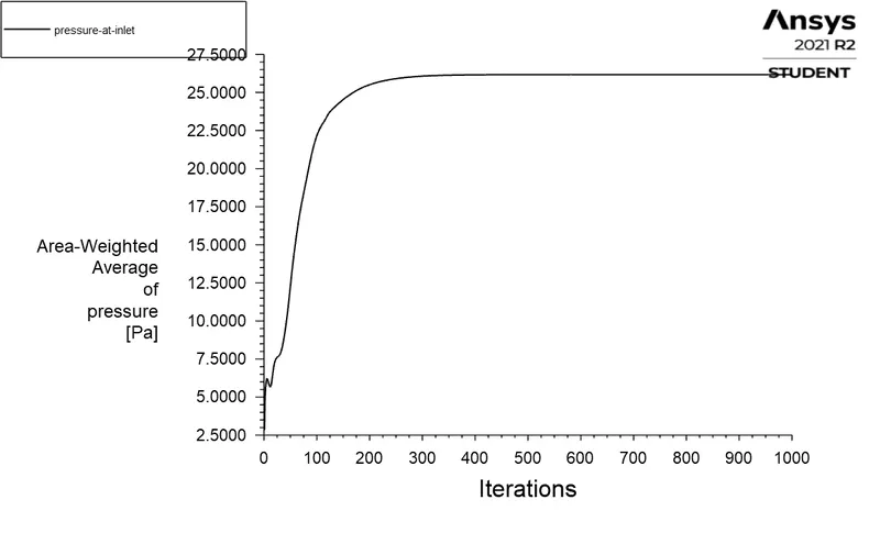
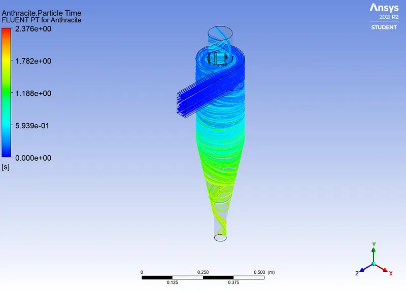
• Case 4 (Velocity = 4m/s)

Part 2 Case 4 Animation

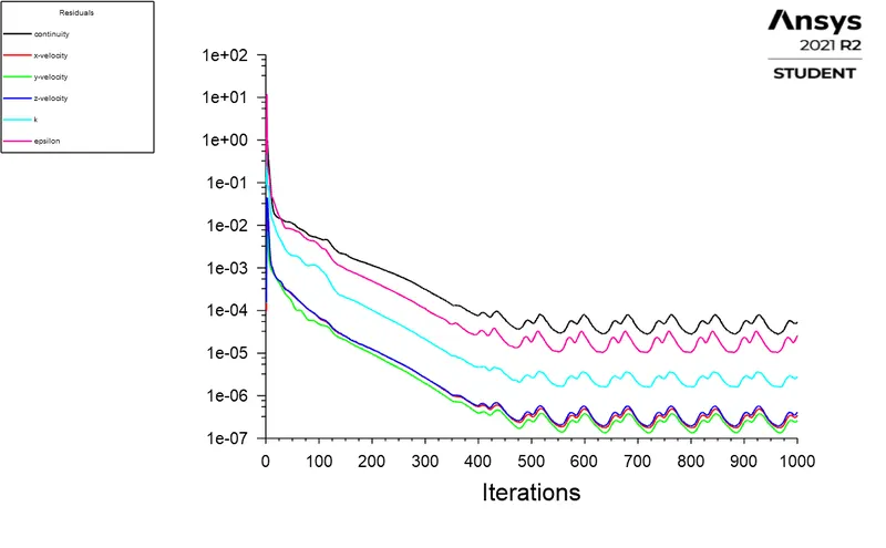
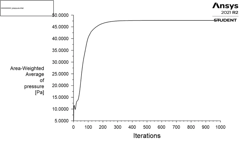
• Case 5 (Velocity = 5m/s)

S. No	Inlet pressure	Outlet 1 pressure
1	26.175342	-0.021032871
2	26.175342	-0.021032871
3	26.175342	-0.021032871
4	26.175342	-0.021032871
5	26.175342	-0.021032871
6	2.2740466	-0.00070138096
7	11.333888	-0.007810081
8	26.175342	-0.021032871
9	47.722241	-0.041875288
10	76.126313	-0.070372395

Part 1	Size of particle (μm)	Velocity of particle(m/s)	Particle tracked	Particle escaped	Particle trapped	Separation efficiency (%)
Case 1	1	3	378	148	230	60.85
Case 2	2		378	121	257	67.99
Case 3	3		378	84	294	77.78
Case 4	4		378	75	303	80.16
Case 5	5		378	73	305	80.69

Part 2	Size of particle (μm)	Velocity of particle(m/s)	Particle tracked	Particle escaped	Particle trapped	Separation efficiency (%)	Pressure drop (Pa)
Case 1	5	1	378	87	291	76.98	2.2740466
Case 2		2	378	71	307	81.21	11.333888
Case 3		3	378	73	305	80.69	26.175342
Case 4		4	378	62	316	83.60	47.722241
Case 5		5	378	67	311	82.28	76.126313

Discussion

The results obtained from the simulations are displayed above. These results are summarized in the above tables. From these tables, it can be seen that, in Part 1, the efficiency of separation increases with the increase in particle size or diameter. And in Part 2, the efficiency also increases with increase in velocity.

Another remark is that in Part 1, the separation efficiency is increasing gradually with particle size; while in Part 2, the separation efficiency increases rapidly as the velocity is incremented. This happens because the impact of pressure drop on cyclone efficiency is an important parameter to be considered.

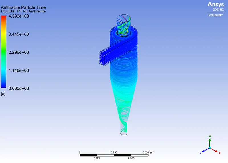
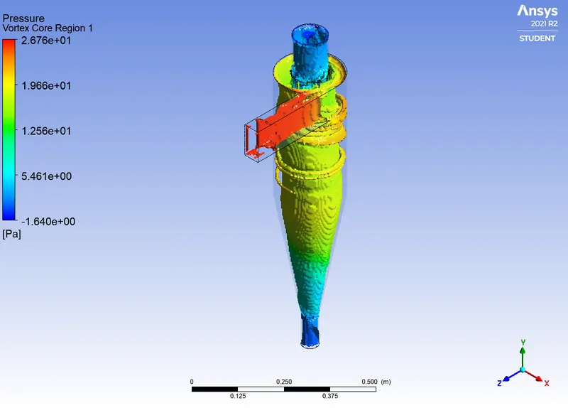
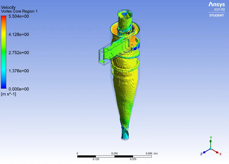
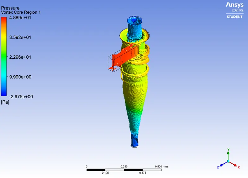
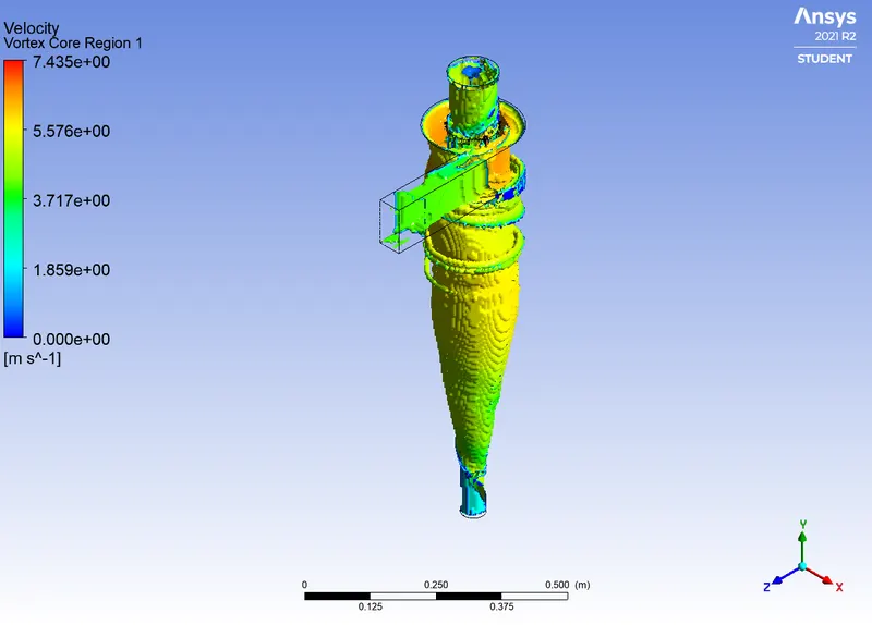
By looking to the different contours, we can see that the pressure as well as the velocity are higher at the inlet compared to the other locations. As for velocity, this is explained by the fact that, particles are being forcefully injected from the inlet. As far as the pressure is concerned, it is also higher at the outer surface and this is because the particles travelling is a swirl motion, are being imparted on the outer surface of the cyclone; hence the particle are projected from axial to radial direction leading to higher pressure drop at the outer surface.

Conclusion

Finally, analysis on cyclone separator is performed throughout ten simulation cases imparted into two. The separation efficiency as well as the pressure drop are calculated and results are discussed. We found that the separation efficiency of a cyclone separator depends on both the particles diameter and their velocity. Considering the results from Part 2, we can conclude that, the particles velocity is the most effective variable to be achieve higher efficiency. Moreover, we determined that, the efficiency of cyclone separator has direct effect on the pressure drop and thereby the higher the velocity, higher the pressure drop and higher the separation efficiency.

References

• Numerical study of gas-liquid flow in a cyclone separator, B. Wang, D.L. Xu, K.W. Chu, A.B. Yu
• A CFD study on the Prediction of Cyclone Collection Efficiency, Jolius Gimmbum, Thomas S. Y. Choong, T.G. Chuah, and A. Fakhru’I-Razi