Otto-cycle Engine Kinematics in Python

AIM: To write a Python program to plot p-v diagram and determine the thermal efficiency of the engine.

OBJECTIVE:

• Understand the different processes of otto-cycle
• Understand how the work is done between gas and piston during each process
• Understand the assumptions made between the reality and ideal otto-cycle
• Understand the behaviour or nature of the curve during each process
• Plot the pressure and volume characteristics (P-V diagram)
• find the thermal efficiency of the engine

INPUTS:

• gamma = adiabatic index
• stoke = stroke length of the connecting rod
• bore = bore diameter of the cylinder
• con_rod = length of the connecting rod
• cr = compression ratio
• v_swept = swept volume of the cylinder
• v_clearance = clearance volume of the cylinder
• theta = crank angle
• v = volume of the cylinder
• e = thermal efficiency of the engine
• p1,v1,t1 = corresponding pressure,volume and temperature at point 1
• p2,v2,t2 = corresponding pressure,volume and temperature at point 2
• p3,v3,t3 = corresponding pressure,volume and temperature at point 3
• p4,v4,t4 = corresponding pressure,volume and temperature at point 4

EQUATIONS USD:

1. v_swept = (pi/4)*bore^2*stroke
2. v_clearance = v_swept/(cr-1)
3. constant_c = p*v^gamma
4. p*v = constant_c*t
5. a = stroke/2
6. R = con_rod/a
7. v/v_c = (1 + 0.5*(cr-1)*(R + 1 - cos(theta) -( R^2 -sin(theta))^0.5))
8. e = 1- 1/[cr^(gamma-1)]

THEORY:

An Otto cycle is an idealized thermodynamic cycle that describes the functioning of a typical spark ignition piston engine. The Otto cycle is a description of what happens to a mass of gas as it is subjected to changes of pressure, temperature, volume, addition of heat, and removal of heat through the following four internally reversible processes:

1. Isentropic compression
2. Constant-volume heat addition

• Isentropic expansion

1. Constant -volume heat rejection

DETAILS:

Programming language used: Python

Concept used: Gas laws, engine kinematics

ASUMPTIONS:

• It is assumed that all the processes are internally reversible
• The working fluid is air, which continuously circulates in a closed loop (cycle).
• Air is considered as ideal gas.
• Combustion process is modelled by a heat-addition process from an external
  source.
• The exhaust process is modelled by a heat-rejection process that restores the
  working fluid (air) at its initial state.
• It is assumed that there will be no inefficiency during isentropic compression and expansion

PROGRAM AND STEPWISE EXPLANATION:

"""
Otto cycle simulator

"""

import matplotlib.pyplot as plt
import math

#""""""""""""""""""""""""""""""""""""""""""""""""""""""""""""""""""""""""""""""""""
#Function definition

def engine_kinematics(bore, stroke, con_rod, cr, start_crank, end_crank):
	

	"""

	Engine Kinematics

	"""
	# Geometric parameters

	a = stroke/2
	R = con_rod/a

	# Volume parameters
	v_s = math.pi*(1/4)*pow(bore,2)*stroke
	v_c = v_s/(cr-1)

	sc = math.radians(start_crank)
	ec = math.radians(end_crank)

	num_values = 1000
	dtheta = (ec - sc)/(num_values - 1)

	v = []


	for i in range(0,num_values):

		theta = sc + i*dtheta
		term1 = 0.5*(cr-1)
		term2 = R + 1 - math.cos(theta)
		term3 = pow( (pow(R,2) - pow(math.sin(theta),2)),0.5)

		v.append((1 + term1*(term2 - term3))*v_c)
	return v

#End of the function
#""""""""""""""""""""""""""""""""""""""""""""""""""""""""""""""""""""""""""""""

# Inputs

p1 = 101325
t1 = 500
gamma = 1.4
t3 = 2300
# Geometric parameters

bore = 0.1
stroke = 0.1
con_rod = 0.15
cr = 5



#Volume computation

v_s = (math.pi/4)*pow(bore,2)*stroke
v_c = v_s/(cr-1)
v1 = v_c + v_s

#State point 2

v2 = v_c


#p2v2^gamma = p1v1^gamma

p2 = p1*pow(v1,gamma)/pow(v2,gamma)

#print(p2)

# p2v2/t2 = p1v1/t1 | rhs = p1v1/t1 |t2 = p2v2/rhs

rhs = p1*v1/t1
t2 = p2*v2/rhs
#Calling the function to calculate the compression volume
v_compression = engine_kinematics(bore, stroke, con_rod, cr,180,0)

constant = p1*pow(v1,gamma)

#Computing the compression pressure
P_compression = []

for v in v_compression:
	P_compression.append(constant/pow(v,gamma))
	

#State point 3

v3 = v2

#p3v3/t3 = p2v2/t2 |rhs = p2v2/t2 | p3 = rhs*t3/v3

rhs = p2*v2/t2
p3 = rhs*t3/v3

#Calling the function to calculate the expansion volume
v_expansion = engine_kinematics(bore, stroke, con_rod, cr,0,180)

constant = p3*pow(v3,gamma)
#Computing the expansion pressure
P_expansion = []

for v in v_expansion:
	P_expansion.append(constant/pow(v,gamma))

# State pointt 4

v4 = v1

#p4v4^gamma = p3v3^gamma

p4 = p3*pow(v3,gamma)/pow(v4,gamma)

# p4v4/t4 = rhs

t4 = p4*v4/rhs

# Calculation of thermal efficiency Therm_eff

Therm_eff = 1 - (1/(pow(cr,(gamma-1))))
print('Efficiency of Otto-Cycle =',Therm_eff)


#Plotting part
plt.figure(1)
plt.plot([v1,v2,v3,v4,v1],[p1,p2,p3,p4,p1])
plt.xlabel("Volume in m^3")
plt.ylabel("Pressure in Pa")
plt.title("P-V Diagram of Otto Cycle engine")

plt.figure(2)
plt.plot([v2,v3],[p2,p3])
plt.plot(v_compression,P_compression)
plt.plot(v_expansion,P_expansion)
plt.plot([v4,v1],[p4,p1])
plt.xlabel("Volume in m^3")
plt.ylabel("Pressure in Pa")
plt.title("P-V Diagram of Otto Cycle engine")
plt.show()

STEPWISE EXPLANATION

As it can be seen, the program above comprises 4 main parts. The first part is about importing the modules or libraries that are relevant for successful running of the code. Thus, the “matplotlib.pyplot” library is imported under the name “plt”. The “math” module is also imported. The second part of this code is about the function definition namely “engine_kinematics”. This function takes bore, stroke, connecting rod, compression ratio, starting crank angle and ending crank angle respectively as arguments. Using the equation 7 stated above, the volume is computed under a “for loop” and stored in an empty array variable with the help of “append” command. The function is instructed to return the value of the computed volume.

The third part of this code is the body of the program where the pressure, the volume as well as the thermal efficiency of the engine are computed for different state points. Firstly, in this part, the useful inputs are defined; then the volume at the isentropic compression as well as isentropic expansion and the pressure are calculated using appropriate formulae as shown in the code.

After that comes the last part of this code which is about plotting the p-v diagram of the otto-cycle engine.

Output:

The output is shown below

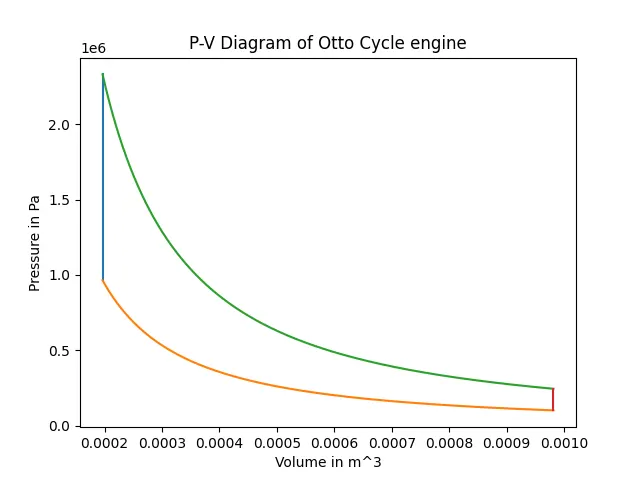
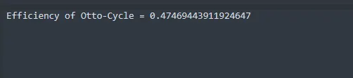
Errors encountered during coding

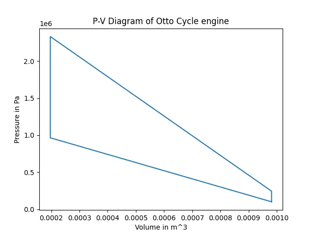
As it can be seen on the graph below, the obtained p-v diagram is wrong. The variation of volume in isentropic compression and isentropic expansion does not vary linearly. Hence the use of equation 7 to properly compute the variation of the volume.

Conclusion:

Finally, a Python code is written to plot the p-v diagram of Otto-cycle engine. The thermal efficiency of the engine is also computed and through this work we are able to understand the behaviour of the curve during each process.