Finite Volume Method Literature Review
What is Finite Volume Method (FVM)?
Generally, we can say that, finite volume method is a numerical method in which the discretization of the field equations of a problem is done by subdividing the problem domain into cells and then writing the field equations in their integral form. In other words, the finite volume method is a discretization method that used the approximation of a single or a system of partial differential equations (PDEs).
Like the finite element method, the mesh consists of partitions of the domain that hosts the space variables. But in the FVM, the elements composing the mesh are termed as control volume and the integration of the PDE over each control volume results in a balance equation. The obtained balance equations are then discretized with respect to discrete unknowns.
One crucial aspect is the discretization of the fluxes at the boundaries of each control volume. So, for FVM to be an efficient method, the numerical fluxes are conservative and consistent. Conservative fluxes means that the quantity of flux entering a control volume is equal to quantity of flux leaving that control volume and consistent means that the numerical flux of a regular function interpolation tends to the continuous flux as the mesh size tends to zero.
However, depending on the problem under study, it might be possible to discretize the fluxes at the boundaries of the control volume by the finite difference method (FDM). But the specificity of the FVM with respect to the FDM is that the discretization is performed on the local balance equations, rather than the PDE. This means that the fluxes on the boundaries of the control volumes are discretized, rather than the continuous differential operator.
Moreover, the advantage of the finite volume method is its easy formulation to allow the unstructured meshes hence the FVM method is used many CFD packages.
In order to explain the steps involved in finite volume method, 1D linear heat conduction equation `∂/(∂x )(α (∂T)/(∂x))+s=0` is used.
In this equation,
`α` represents the thermal diffusivity,
`(∂T)/(∂x)` represents the temperature gradient in x direction and
s is the source term.
This governing equation is valid at each point in the whole domain hence it is valid for the entire control volume.
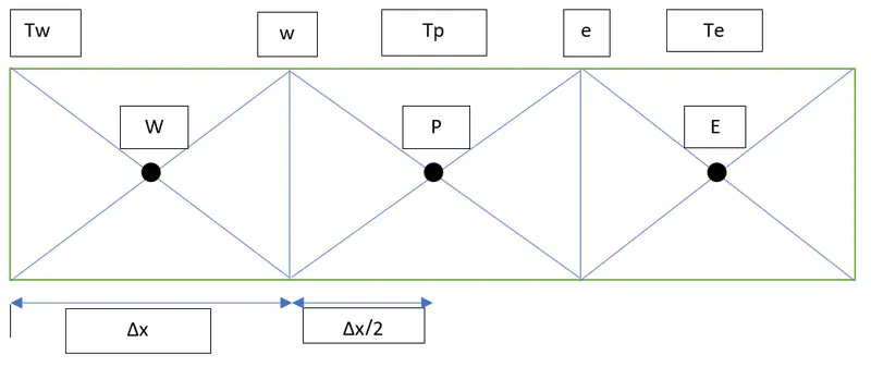
As discussed earlier, the integral form of the governing equations are used in finite volume method. So, in order to get that form, a small control volume (dv) as shown below in the figure is multiplied with the governing equation and integrated for the entire volume.
The following equation is obtained:
`∫(∂/(∂x) (α (∂T)/(∂x))+s)dv=0`
`∫(∂/(∂x) (α (∂T)/(∂x)))dv+∫sdv=0`
dv= A*dx where A is the Area.
`∫(∂/(∂x) (α ∂T/(∂x)))Adx+∫sdv=0`
`[αA(∂T/∂x)]_w^e+ s ̅dv=0`
`s ̅`is considered to be the average value of the source term s.
`α_e A[(T_e-T_p)/(∆x)]-α_w A[(T_p-T_w)/(∆x)]+ s ̅dv=0`
Since, the thermal diffusivity is a function of temperature, if it is considered to be constant, we get the following equation:
`αA[(T_e-T_p)/(∆x)]-αA[(T_p-T_w)/(∆x)]+ s ̅dv=0`
In case when the thermal diffusivity is not constant, then it should be linearized as follows:
`s ̅dv□(→┴Linearization ) S_u+S_p T_p`
`[Heatflux]_out-[Heatflux]_in+Sourceterm=0`
What is the need of Interpolation Scheme?
In order to understand the interpolation schemes, it urges to know first what is interpolation. Thus, interpolation is a statistical method used to estimate the values at unknown points. It is achieved by using other established or known values that are located in sequence with the unknown values.
Interpolation schemes are used in transformation of cell-centre quantities to face centres. This operation is mostly encountered in finite volume calculations such as gradient, divergence and Laplacian calculations.
However, there several interpolation schemes used in finite volume method.
- Upwind interpolation scheme (USD)
- Linear interpolation scheme
- Quadratic Upwind interpolation scheme
- Hybrid interpolation scheme
- Total variation diminishing scheme
- Essentially non-oscillatory interpolation scheme
What is the need of flux limiters?
Flux limiters are used in high resolution schemes to avoid the spurious oscillations that would otherwise occur with high order spatial discretization schemes due to shocks, discontinuities or sharp changes in the solution domain.
The idea is to tune the numerical flux of high order and low order scheme using the flux limiter function in such a way that the resulting scheme gives a high order accuracy in the smooth region of flow and sticks with first order of accuracy in the vicinity of shocks or discontinuities as follows:
`F_(j+1/2)=L_(j+1/2)+∅(H_(j+1/2)-L_(j+1/2) )` where L, H are the numerical flux of conservative low order and high order schemes respectively. `∅` is a function of smoothness parameter `θ` usually defined as `θ_j= (U_j-U_(j-1))/(U_(j+1)-U_j )`
He next step is to define the limiter function `∅(θ)` in such a way that it satisfies at least the following properties:
- Remains positive Ɐθ
- Satisfies ф (1) = 1
- Passes through a particular region known as TVD region associated with the underlying scheme in order to guarantee stability of the scheme.
REFERENCES: