Genetic Algorithm

AIM: To write a MATLAB program to optimise the stalagmite function and find the global maxima of the function.

OBJECTIVE:

• Understand and explain the concept of Genetic Algorithm
• Master and explain the ga syntax in MATLAB
• To learn how to use Genetic Algorithm to optimise a function

EQUATIONS USED:

`f_1=(sin(5.1*π*x+0.5))^6`

`f_2=(sin(5.1*π*y+0.5))^6`

`f_3=e^((-4 log⁡2*(x-0.0667)^2)/(0.64))`

`f_4=e^((-4 log⁡2*(y-0.0667)^2)/(0.64))`

`F=-(f_1*f_2*f_3*f_4)`

THEORY:

During problem-solving, one looks for the best results which can be only achieved by a decision-making process under certain major criteria or principles. Such procedure is namely called optimisation; and since its objective is to get an optimum or satisfactory solution, it is executed by comparing various solutions.

To perform the optimisation, there are methods such as deterministic method and stochastic method: Deterministic method makes use of specific rules for moving one solution to another; the Stochastic method possesses some inherent randomness, it is a probabilistic approach which requires to choose an optimisation algorithm while performing optimisation.

Genetic Algorithm which is an example of optimisation algorithm, can be used to solve both constrained and unconstrained optimisation problems. It is based on natural selection, the process that drives biological evolution. The genetic algorithm repeatedly modifies a population of individual solutions.

The genetic algorithm in order to create the next generation from the current population, uses three main types of rules:

• Selection rules: select the individuals called parents that contributes to the next generation
• Crossover rules: combine two parents to form children for the next generation
• Mutation rules: apply random changes to individual parents to form children

SYNTAX OF GENETIC ALGORITHM (ga)

x = ga(fun,nvars)

x = ga(fun,nvars,A,b)

x = ga(fun,nvars,A,b,Aeq,beq)

x = ga(fun,nvars,A,b,Aeq,beq,lb,ub)

x = ga(fun,nvars,A,b,Aeq,beq,lb,ub,nonlcon)

x = ga(fun,nvars,A,b,Aeq,beq,lb,ub,nonlcon,options)

x = ga(fun,nvars,A,b,[],[],lb,ub,nonlcon,IntCon)

x = ga(fun,nvars,A,b,[],[],lb,ub,nonlcon,IntCon,options)

x = ga(problem)

[x,fval] = ga(___)

[x,fval,exitflag,output] = ga(___)

[x,fval,exitflag,output,population,scores] = ga(___)

Explanation of the Syntax

Through the above syntax, we can clearly see the input arguments and output arguments as well:

• Inputs

• fun: is the objective function
• nvars: is the dimension or the number of the design variables of the function fun
• A: is the linear inequality constraint
• b: is the linear inequality constraint
• is the equality constraint
• is the equality constraint
• lb: lower bound
• ub: upper bound
• nonlcon: Nonlinear constraint
• options: Stock of integer variables
• Intcon: integer variables
• problem: is the structure

• Outputs

• x: is the solution
• fval: is the value of fitness function at x
• exitflag: is the integer value identifying the reason the algorithm terminated
• output: is structure that contains output from each generation
• population: matrix giving final population
• scores: is the scores of the final population

MATLAB PROGRAM:

clear all
close all
clc

% Defining our search space
x = linspace(0,0.6,150);
y = linspace(0,0.6,150);
iterations = 40

% Creating a 2 Dimensional mesh
[xx yy] = meshgrid(x,y);

% Evaluating the stalagmite function
for i = 1:length(xx)
    for j = 1:length(yy)
        input_vector(1)=xx(i,j);
        input_vector(2)=yy(i,j);
        f(i,j) = stalagmite(input_vector);
    end
end

%First iteration
%At this level we will study the statistical behaviour
tic
for i = 1:iterations
    [inputs,foptimum(i)] = ga(@stalagmite,2);
    xoptimum(i) = inputs(1);
    yoptimum(i) = inputs(2);
    
end
First_iteration_time = toc

%Plotting

figure(1)
subplot(2,1,1)
hold on
surfc(xx,yy,-f)
xlabel('x value');
ylabel('y value');
shading interp
plot3(xoptimum,yoptimum,-foptimum,'marker','o','markersize',7,'markerfacecolor','g')
title('Unbounded inputs')
subplot(2,1,2)
plot(-foptimum)
xlabel('Iterations')
ylabel('Function Maximum')

%Second iteration
%In this iteration the lower limit and the upper limit are fixed
tic
for i = 1:iterations
    [inputs,foptimum(i)] = ga(@stalagmite,2,[],[],[],[],[0;0],[1;1]);
    xoptimum(i) = inputs(1);
    yoptimum(i) = inputs(2);
    
end
Second_iteration_time = toc
    
%Plotting

figure(2)
subplot(2,1,1)
hold on
surfc(xx,yy,-f)
xlabel('x value');
ylabel('y value');
shading interp
plot3(xoptimum,yoptimum,-foptimum,'marker','o','markersize',7,'markerfacecolor','g')
title('Bounded inputs')
subplot(2,1,2)
plot(-foptimum)
xlabel('Iterations')
ylabel('Function Maximum')

%Third iteration
%Here the upper and the lower limits are fixed plus the population size is
%incressed to 300
options = optimoptions('ga')
options = optimoptions(options,'PopulationSize',300);

tic
for i = 1:iterations
    [inputs,foptimum(i)] = ga(@stalagmite,2,[],[],[],[],[0;0],[1;1],[],[],options);
    xoptimum(i) = inputs(1);
    yoptimum(i) = inputs(2);
    
end
Third_iteration_time = toc
    
%Plotting

figure(3)
subplot(2,1,1)
hold on
surfc(xx,yy,-f)
xlabel('x value');
ylabel('y value');
shading interp
plot3(xoptimum,yoptimum,-foptimum,'marker','o','markersize',7,'markerfacecolor','g')
title('Increased population with Bounded inputs')
subplot(2,1,2)
plot(-foptimum)
xlabel('Iterations')
ylabel('Function Maximum')

FUNCTION USED:

function [F] = stalagmite(input_vector)
   x = input_vector(1);
   y = input_vector(2);
   
   
   f1 = (sin(5.1*pi*x + 0.5)).^6;
   f2 = (sin(5.1*pi*y + 0.5)).^6;
   f3 = exp((-4*log(2)*(x-0.0667).^2)/(0.64));
   f4 = exp((-4*log(2)*(y-0.0667).^2)/(0.64));
   F = -f1*f2*f3*f4;
   
end

STEPWISE EXPLANATION OF THE CODE:

As shown above, the whole program comprises two main parts:

• Function part

In this part we have created a function called stalagmite using standard formulae within MATLAB.

This function is computed based on the equation shown previously.

Since we are supposed to use the genetic algorithm for the optimisation of the stalagmite function that we created, one can notice that a negative sign is present on the last line of the function code. This is because genetic algorithm intends to determine the minimum of the function. So to get proper output, it is best to use that negative sign.

• Main program

This main program is subdivided into different parts as follows:

• Starting block

This part as its name suggested, is about the freeing the memory from all previous content. It especially makes use of following commands: clear all, close all, clc.

• Definition of the search space

This block of our code uses the linspace command which let us define the values of x and y. As it is shown in the code, x and y take 150 different values each between 0 and 0.6; and as it can be seen the number of iterations is set to 40 which means that the program will run 40 times.

• Creation of the mesh

Under this block, we use meshgrid command to create a 2D mesh taking the values of x and y previously defined as inputs.

• Evaluation of the stalagmite function

At this level, we evaluate the stalagmite function by using For loop.

• Study of different cases

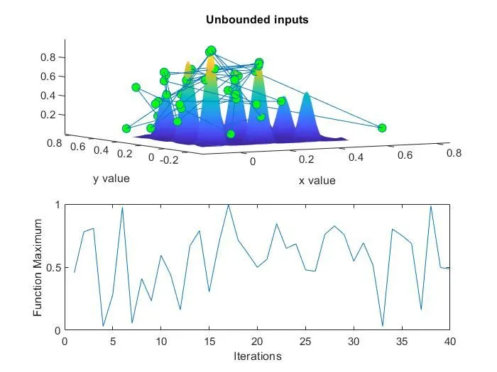
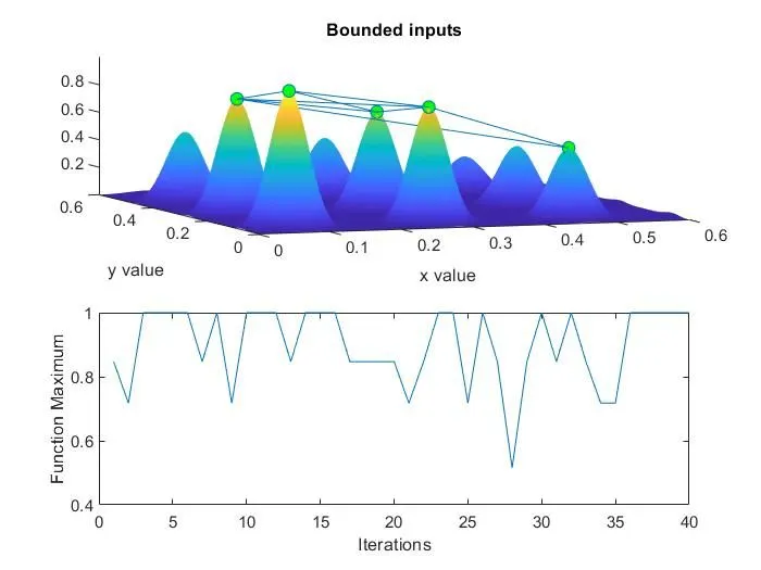
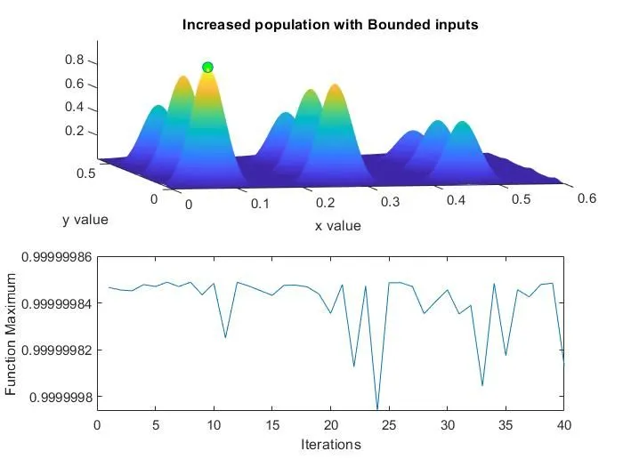
In this block, three cases are carefully studied and the results are shown through the corresponding outputs:

• First case or first iteration

Here the statistical behaviour is studied using for loop. The stalagmite function is called with genetic algorithm (ga) and the corresponding plotting is done. This portion of program uses tic and toc commands to calculate the taken for execution.

• Second case or second iteration

In this part, the statistical behaviour study is carried out under certain constraints. The upper bound and lower bound are fixed. And the same thing is done as in previous case using for loop, stalagmite function, ga, tic and toc commands.

• Third case or third iteration

In this portion, the same study is performed under the same constraints as in the second case plus the fact that here the optimisation function ga is used to increase the population size to 300.

This is done by using ‘options’, ‘optimoptions’ and plotting is done.

OUTPUTS:

• Output for the first study

• output for second study

• output for third study

ERRORS DURING CODING:

As a solution for further cases, we have to in our mind that MATLAB is a case-sensitive programming language.

REFERENCES:

https://in.mathworks.com/help/gads/what-is-the-genetic-algorithm.html

https://towardsdatascience.com/introduction-to-genetic-algorithms-including-example-code-e396e98d8bf3

https://skill-lync.com/knowledgebase/genetic-algorithm-explained