Parametric study on Gate valve.
Aim: To perform a parametric study on the gate valve simulation.
Objectives:
The aim of this project is to carry out a parametric study on the gate valve by setting the opening from 10% to 80% with the objective to:
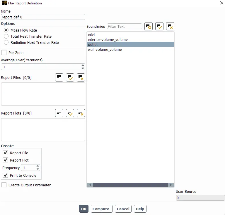
- Obtain the mass flow rates at the outlet for each design point
- Calculate the flow coefficient and flow factor for each opening and plot the graph
- Discuss the results of the mass flow rate and flow coefficient
Introduction
A gate valve also known as a sluice valve, is a valve that opens by lifting a barrier (gate) out of the path of the fluid. Gate valves require very little space along the pipe axis and hardly restrict the flow of fluid when the gate is fully opened. The gate faces can be parallel but are most commonly wedge-shaped (in order to be able to apply pressure on the sealing surface). The work in this project is to perform a parametric study on the above device throughout a simulation in ANSYS Fluent. This is done by creating a parameter in Space Claim with an opening of 10 mm and further, the data for other opening values corresponding to other design points is obtained by updating the parameter.
Theory
As defined above, the gate valves are devices that are used to shut off the flow of liquids rather than for flow regulation. When fully open, the typical gate valve has no obstruction in the flow path, resulting in very low flow resistance. The size of the open flow path generally varies in a nonlinear manner as the gate is moved. This means that rate does not change evenly with stem travel. Gate valves are mostly used with larger pipe diameter since they are less complex to construct than other types of valves in large sizes. At high pressures, friction can become a problem. As the gate is pushed against its guiding rail by the pressure of the medium, it becomes harder to operate the valve. Large gate valves are sometimes fitted with a bypass controlled by a smaller valve to be able to reduce the pressure before operating valve itself. Gate valves without an extra sealing ring on the gate or the seat are used in applications where minor leaking of the valve is not an issue, such as heating circuits or sewer.
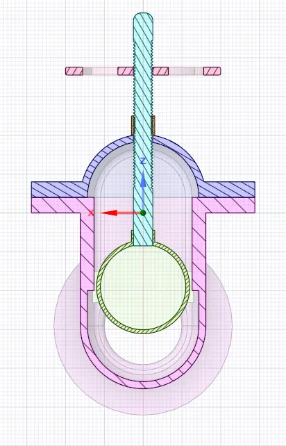
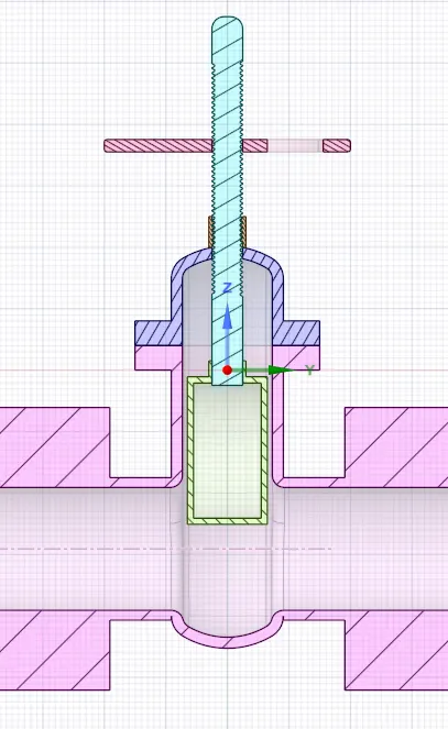
As far as the gate valve structure and working, it is actuated by a threaded stem that connects the actuator (handwheel) to the gate. It is characterized as having either a rising or a nonrising stem, depending on which end of the stem is threaded. Rising stems are fixed to the gate and rise and lower together as the valve is operated, providing a visual indication of valve position. The actuator is attached to a nut that is rotated around the threaded stem to move it. Nonrising stem valves are fixed to and rotate with the actuator and are threaded into the gate. Gate valves are typically constructed from cast iron, cast carbon steel, ductile iron, gunmetal, stainless steel, alloy steels and forged steels. The different components of gate valve are: Bonnet, Pressure seal bonnet, knife gate, the handwheel, the gate disc, the bottom, etc.
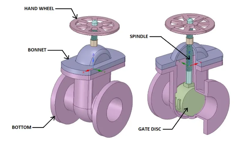
- Modelling and Solving
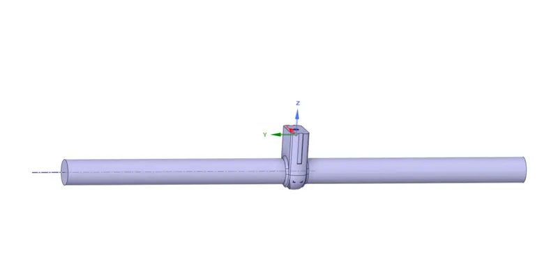
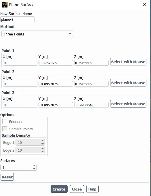
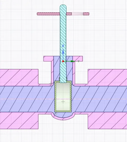
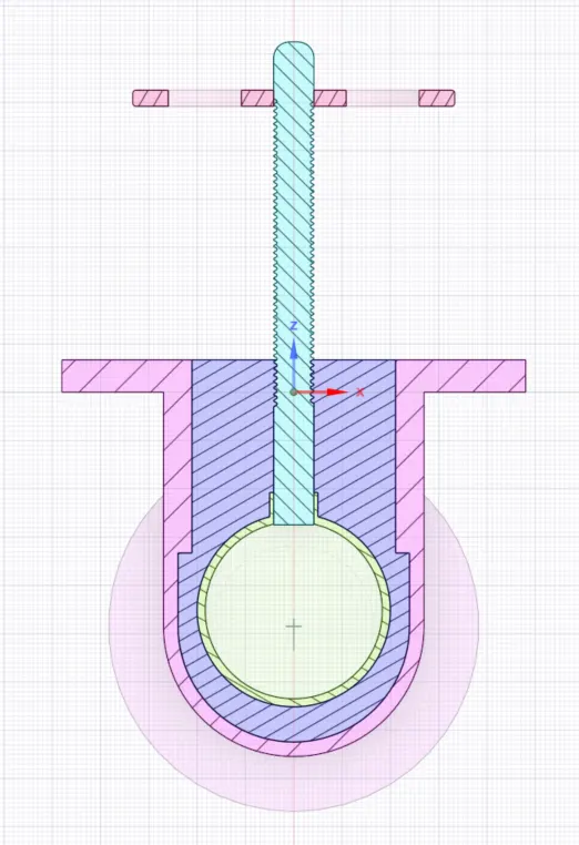
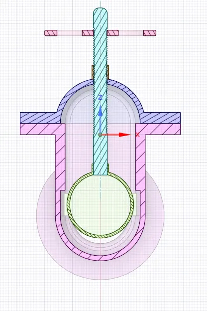
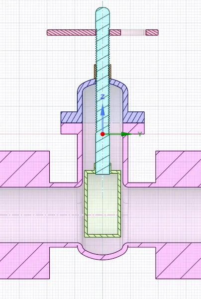
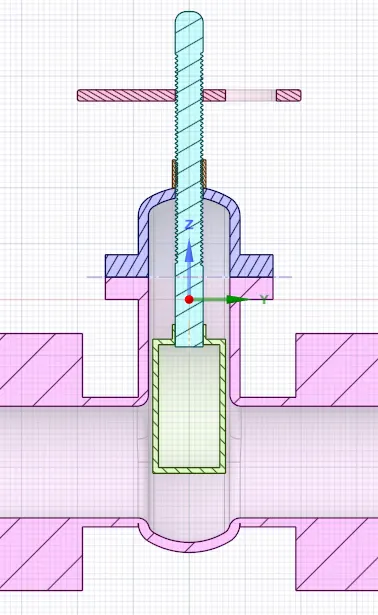
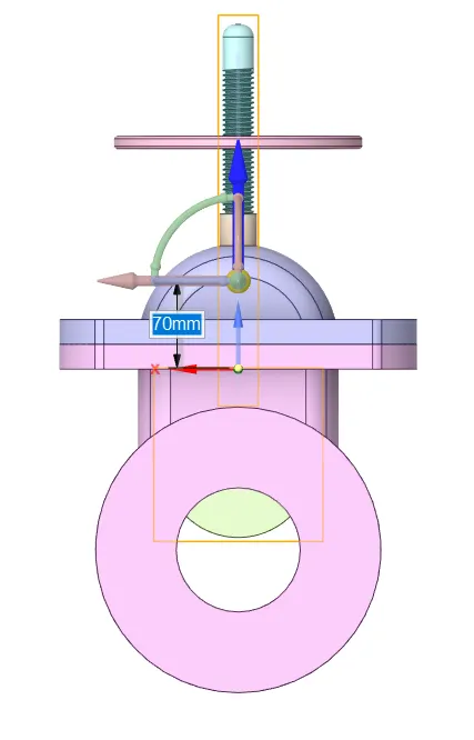
- The CAD model is imported in Space Claim and a rise of 10mm is applied to the gate disc.
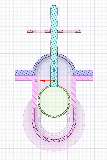
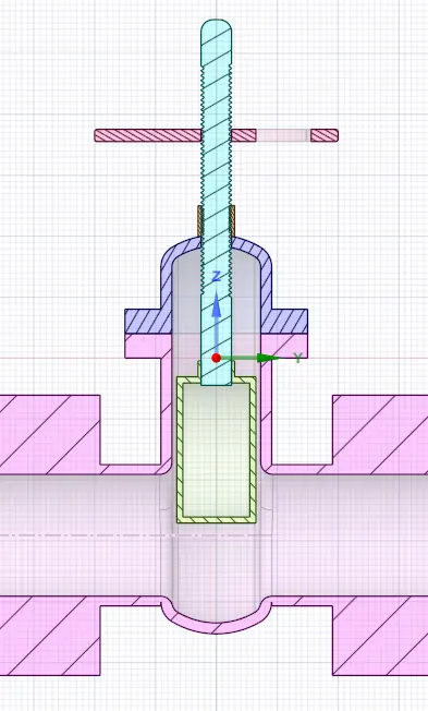
- Then the fluid volume is extracted using “volume extract” command under ‘Prepare’ option. The fluid flow regions at the inlet and outlet are then extend about 800mm using “Pull” command.
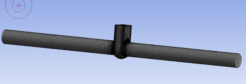
- After that, the model is moved to the meshing module where a named selection is performed after generating a default mesh of 92.892mm size.
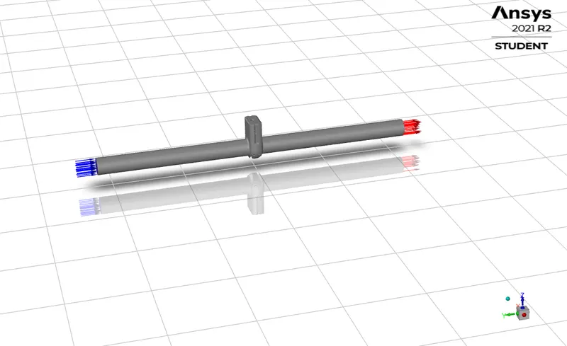
- The model is then transferred to Fluent.
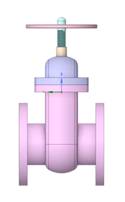
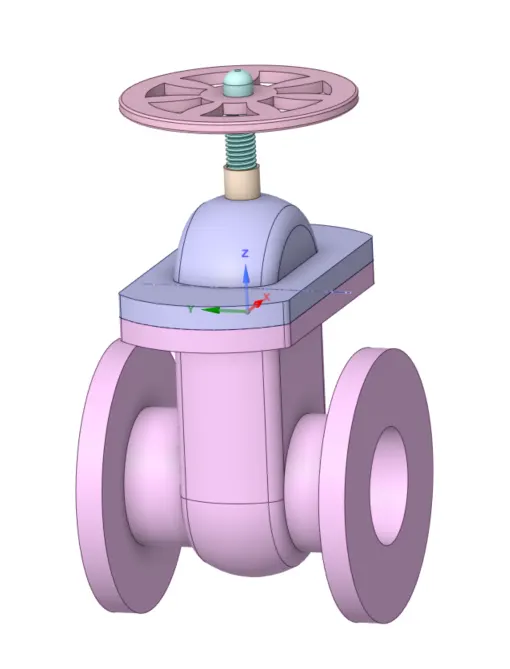
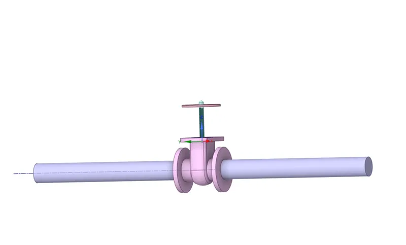
- Setting up the Case (Pre-processing)
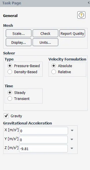
- The gravity is applied in negative z-direction.
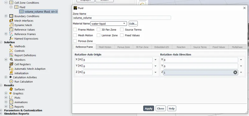
- The fluid is chosen as water-liquid in Fluent database. It is set under cell zone conditions option as the fluid flowing in the fluid volume.
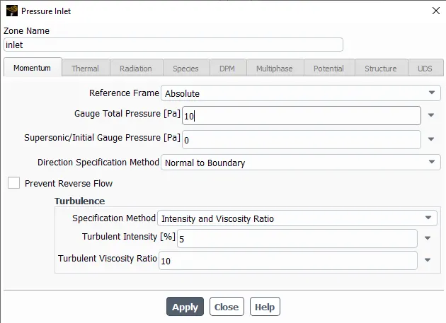
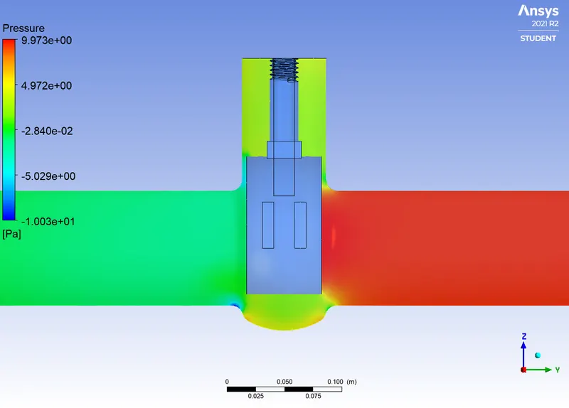
- Now, the boundary conditions are set up. The BC at inlet is set as pressure-inlet with a value of 10 Pa. The other parts remaining by default; that means the outlet is set as pressure-outlet, the interior-volume_volume as interior and the wall-volume _volume as wall.
- The material of fluid flowing in fluid volume is water-liquid with Density=998.2Kg/m3 and Viscosity=0.001003Kg/(m-s).
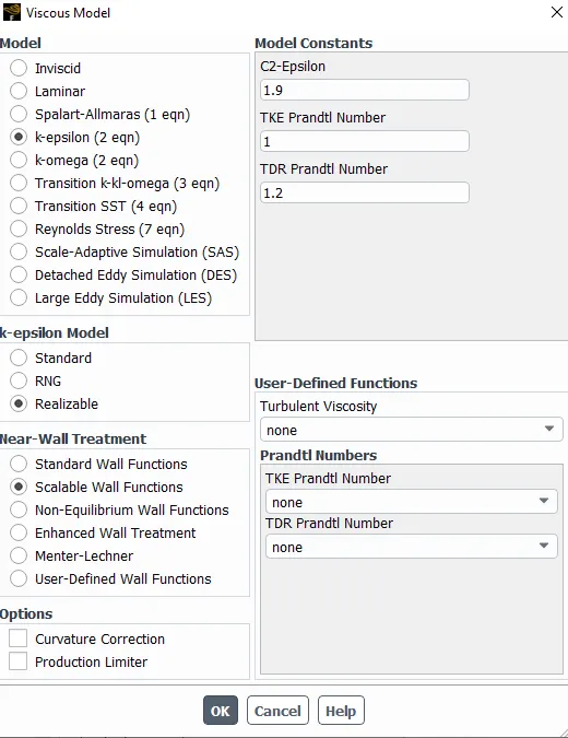
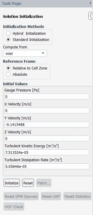
- The viscous model is then defined. The Realisable k-Ꜫ model with Scalable Wall Functions is used. This choice is justified by the calculations below:
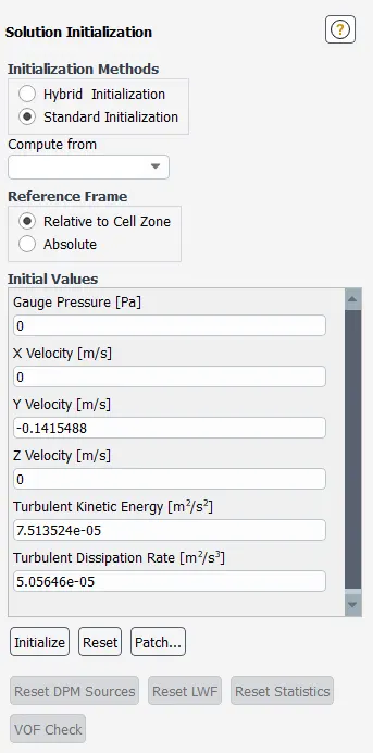
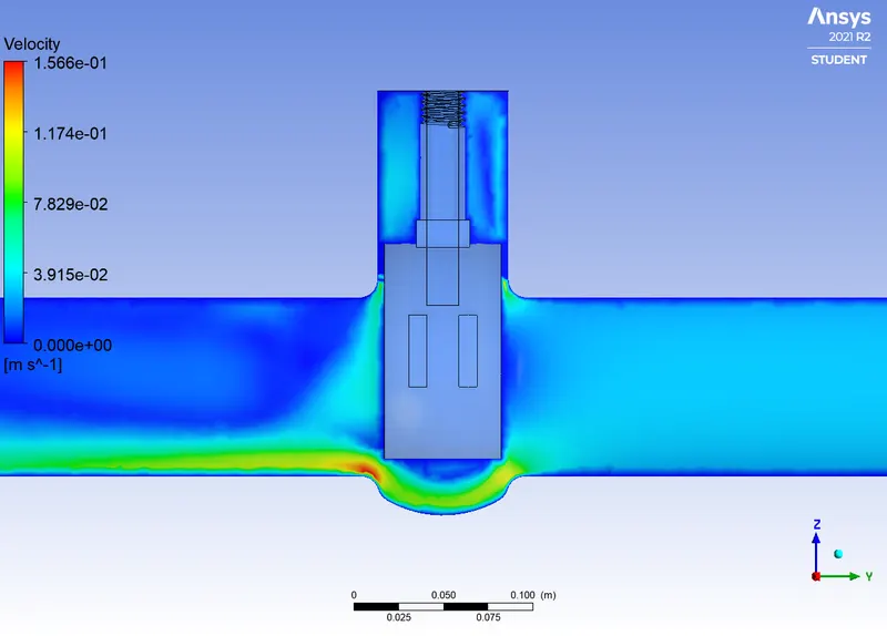
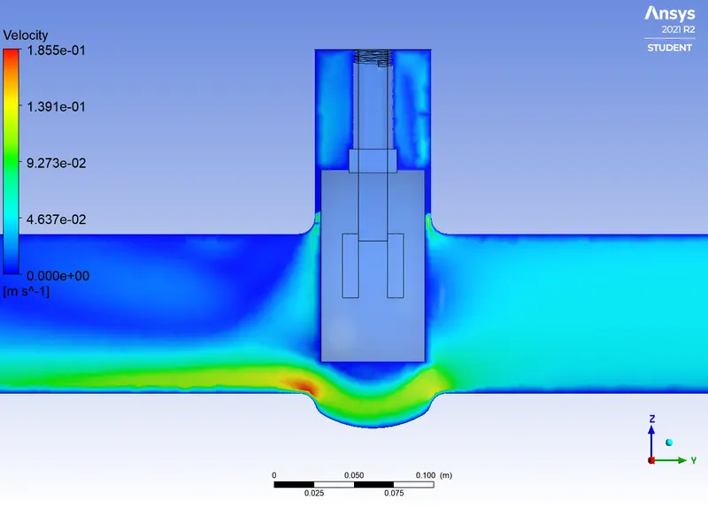
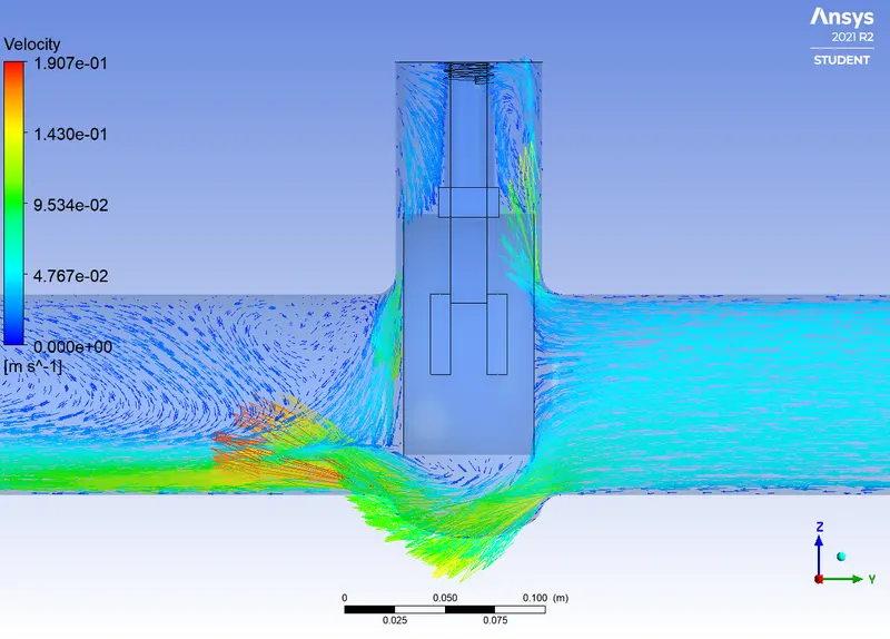
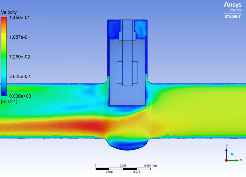
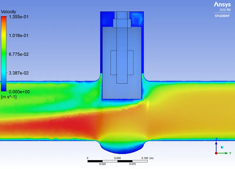
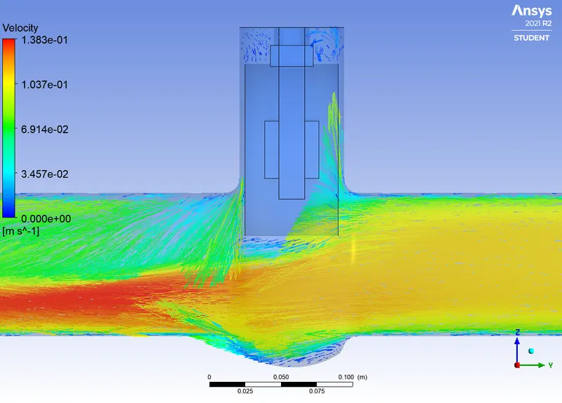
In the facing image, the velocity in y-direction is 0.1415488 m/s. The Reynolds Number is calculated using the following formula: `Re=(ρ×V×D)/μ`. In our case,
`ρ=998.2(Kg)/m^3`
`D=0.1m`
`V=0.1415488 (m)/s`
`Re=(998.2×0.1415488×0.1)/0.001003=14087.14`
From these calculations, the Reynolds Number appears to be greater than 2000 hence the adequate viscous model to be used is k-Ꜫ model.
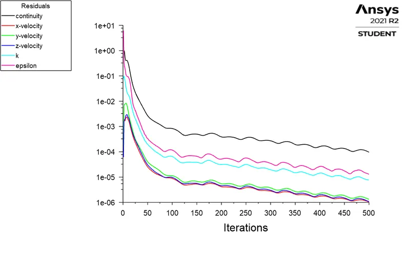
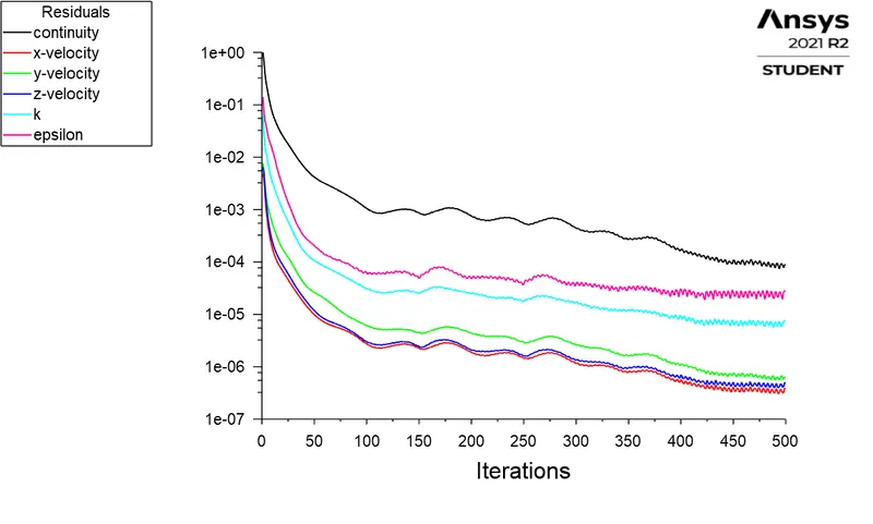
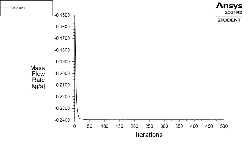
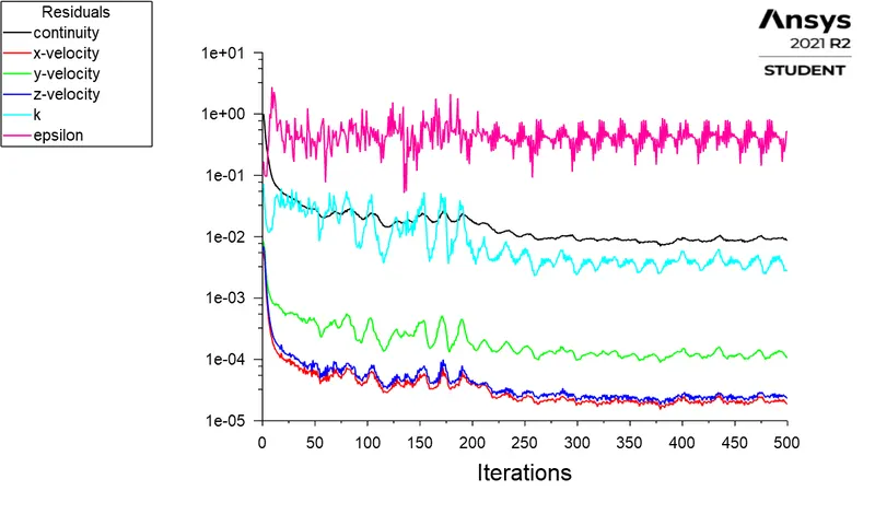
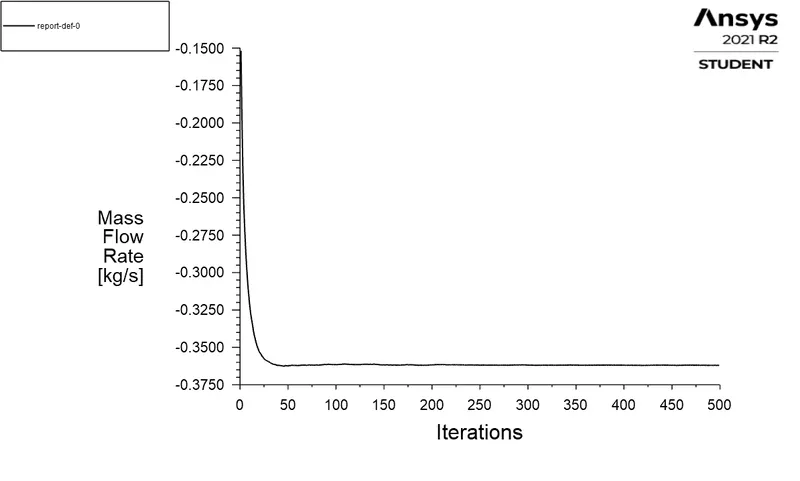
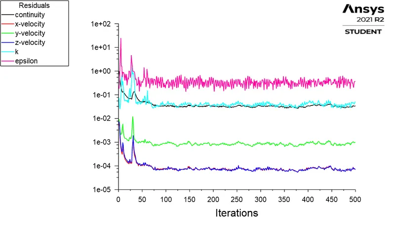
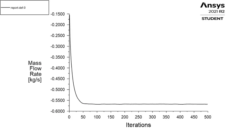
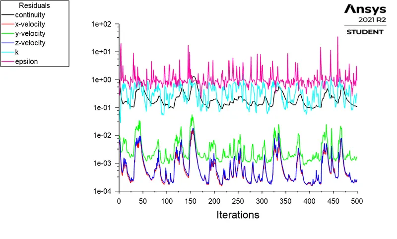
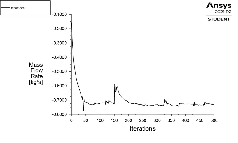
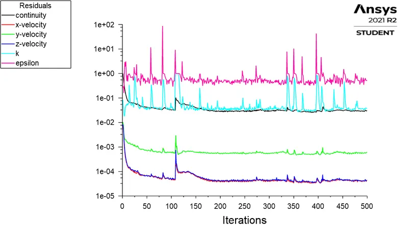
The case is set up using the above specifications and the simulation is run for 500 iterations.
- Mesh refinement
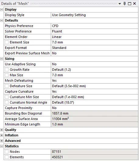
After running the base case successfully, the mesh size is reduced to 7 mm and a new case is set up using the same specifications as stated above.
Mass Flow rate:
In physics and engineering, mass flow rate is the mass of a substance which passes per unit of time. Its unit is kilogram per second in SI units, and slug per second or pound per second in second in US customary units. Mass flow rate is defined by the limit:
`ṁ= (dm)/dt`
Flow Coefficient:
The flow coefficient of a device is a relative measure of its efficiency at allowing fluid flow. It describes the relationship between the pressure dop across an orifice valve or other assembly and the corresponding flow rate.
Mathematically the flow coefficient Cv is expressed as:
`C_v=Q√((SG)/(∆P))`
Where
Q is the rate of flow (expressed in US gallons per minute),
SG is the specific gravity of the fluid (for water=1);
∆P is the pressure drop across the valve (expressed in psi)
Flow Factor:
Flow factor (Kv) is the flow coefficient in metric units that is defined as the flow rate in cubic meters per hour(m3/h) of water at a temperature of 16°C with a pressure drop across the valve or any other restricting device of 1 bar. The Kv is related to the head drop (∆h) or pressure drop (∆P) across the valve with the flow rate (Q).
Mathematically, the Flow Factor is given as:
`K_v=0.865*C_v`
Results
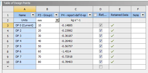
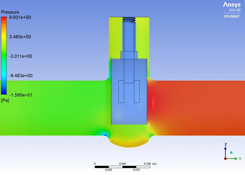
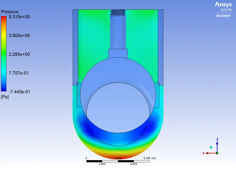
The following results present the eight cases that are the eight design points corresponding each to a lift of the gate disc varying from 10% to 80 %.
The updated parametrization table is given below:
Pressure Drop Calculation
1 Pa = 0.0001450377 Psi
|
Cases |
Pressure at inlet (Pa) |
Pressure at outlet (Pa) |
Pressure drop (Pa) |
Pressure drop (Psi) |
|
Dp0 |
9.8190364 |
0 |
9.8190364 |
0.0014241308 |
|
Dp1 |
9.5302421 |
0 |
9.5302421 |
0.0013822448 |
|
Dp2 |
8.9298693 |
0 |
8.9298693 |
0.001295168 |
|
Dp3 |
9.4342056 |
-0.050969141 |
9.4342056 |
0.0013683158 |
|
Dp4 |
7.3665657 |
0 |
7.3665657 |
0.00106843 |
|
Dp5 |
5.6430005 |
0 |
5.6430005 |
0.000818448 |
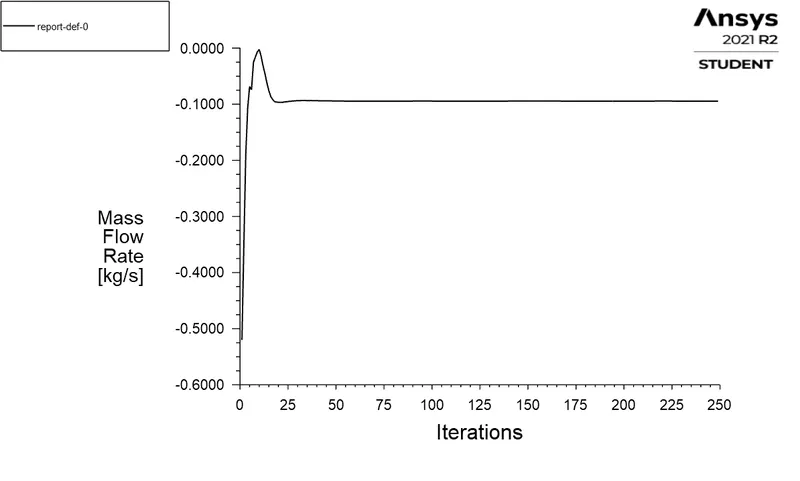
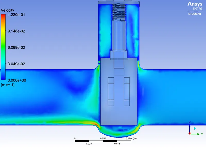
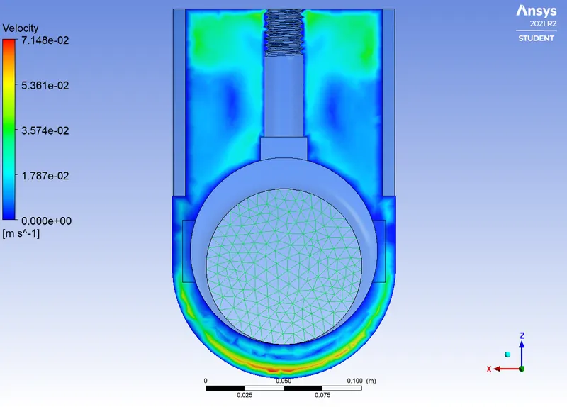
Case 1: Gate disc lift = 10 mm
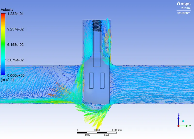
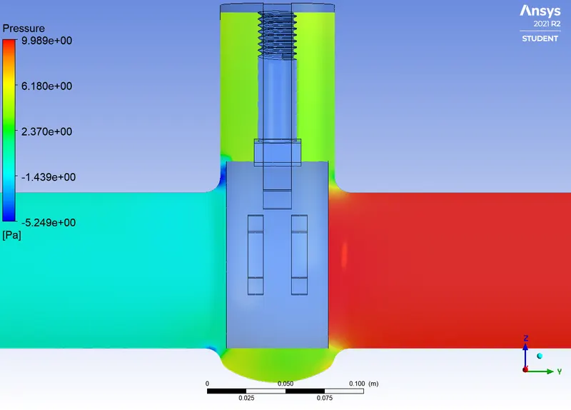
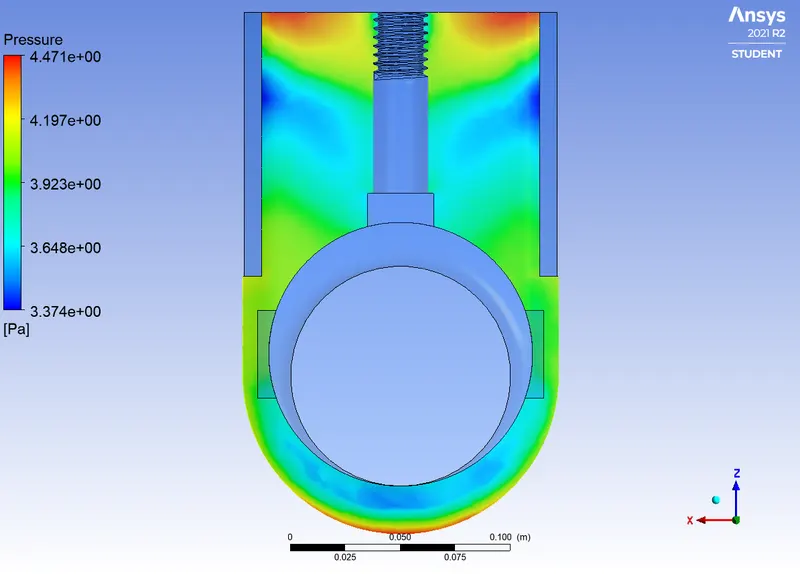

`C_v=Q√((SG)/(∆P))`
Q = 0.14885 kg/s = 2.35932 gal/min
SG = 1000/998.2≈1
∆P= 0.0014241308
`C_v=2.35932√(1/0.0014241308)=62.519`
`K_v=0.865*C_v =>K_v=0.865*62.519=54.0789`
Case 2: Gate disc lift = 20 mm
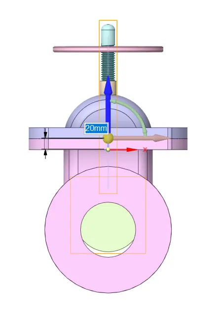
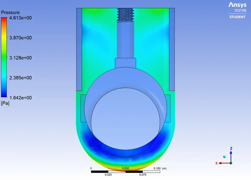

`C_v=Q√((SG)/(∆P))`
Q = 0.23982 Kg/s = 3.80122 gal/min
SG = 1000/998.2≈1
∆P= 0.0013822448
`C_v=3.80122 √(1/0.0013822448)=102.242`
`K_v=0.865*C_v =>K_v=0.865*102.242=88.4393`
Case 3: Gate disc lift = 30 mm
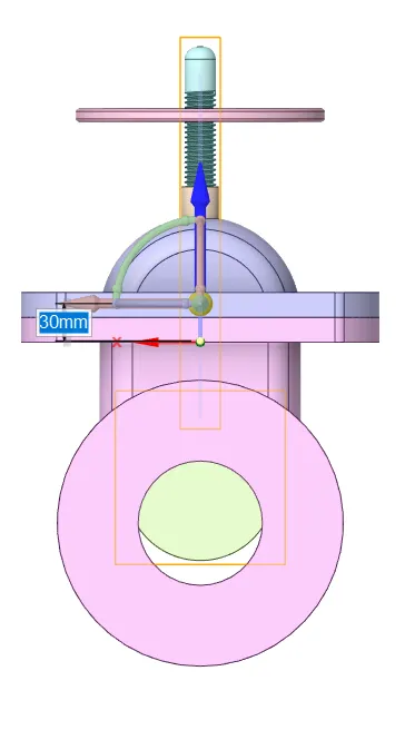
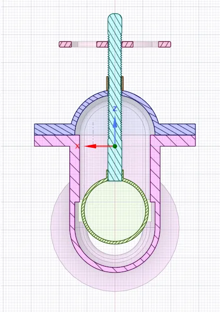
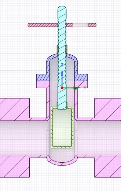

`C_v=Q√((SG)/(∆P))`
Q = 0.36187 Kg/s = 5.73576 gal/min
SG = 1000/998.2≈1
∆P= 0.001295168
`C_v=5.73576√(1/0.001295168)=159.378`
`K_v=0.865*C_v=>K_v=0.865*159.378=137.862`
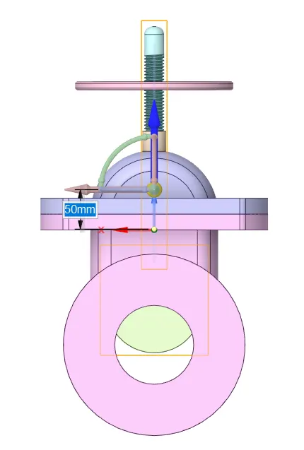
Case 4: Gate disc lift = 50 mm
`C_v=Q√((SG)/(∆P))`
Q = 0.56757 Kg/s = 8.99617 gal/min
SG = 1000/998.2≈1
∆P= 0.00106843
`C_v=8.99617 √(1/0.00106843)=275.223`
`K_v=0.865*C_v =>K_v=0.865*275.223=238.068`
Case 5: Gate disc lift = 70 mm
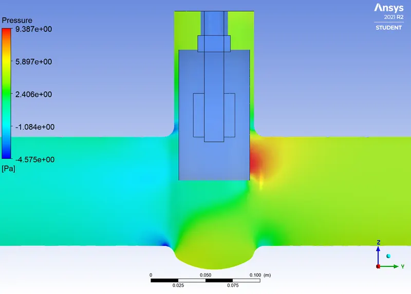
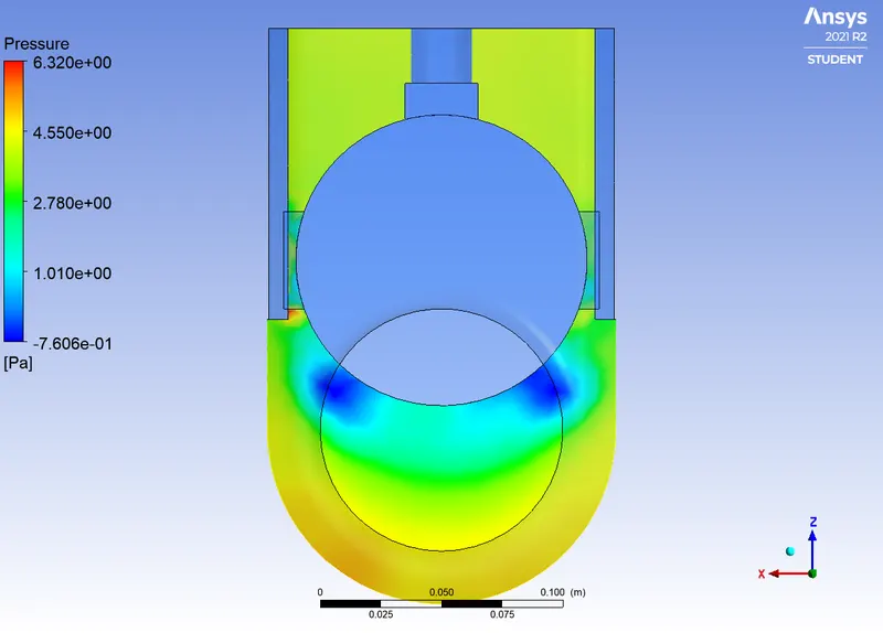

`C_v=Q√((SG)/(∆P))`
Q = 0.72918 Kg/s = 11.55774 gal/min
SG = 1000/998.2≈1
∆P= 0.000818448
`C_v=11.55774 √(1/0.000818448)=403.996`
`K_v=0.865*C_v=> K_v=0.865*403.996=349.457`
Case 6: Gate disc lift = 80 mm
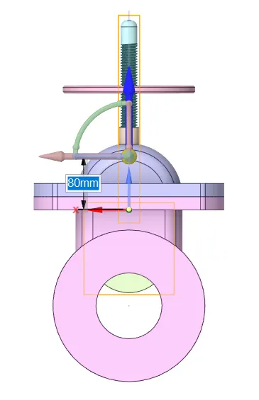
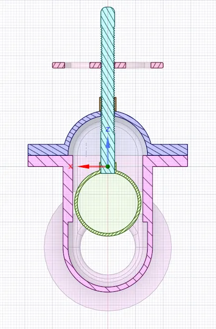

`C_v=Q√((SG)/(∆P))`
Q = 0.78403 Kg/s = 12.42713 gal/min
SG = 1000/998.2≈1
∆P= 0.0007218264
`C_v=12.42713√(1/0.0007218264)=462.546`
`K_v=0.865*C_v=> K_v=0.865*462.546=400.102`
|
Cases Number |
Mass Flow Rate (kg/S) |
Gate Disc lift (mm) |
Flow Coefficient |
Flow Factor |
|
1 |
2.35932 |
10 |
62.519 |
54.0789 |
|
2 |
3.80122 |
20 |
102.242 |
88.4393 |
|
3 |
5.73576 |
30 |
159.378 |
137.862 |
|
4 |
8.99617 |
50 |
275.223 |
238.068 |
|
5 |
11.55774 |
70 |
403.996 |
349.457 |
|
6 |
12.42713 |
80 |
462.546 |
400.102 |
Discussion
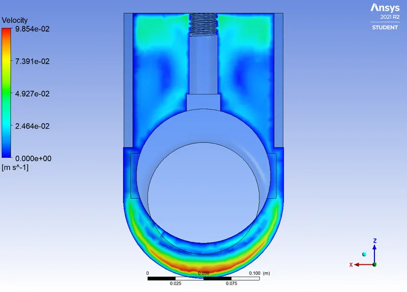
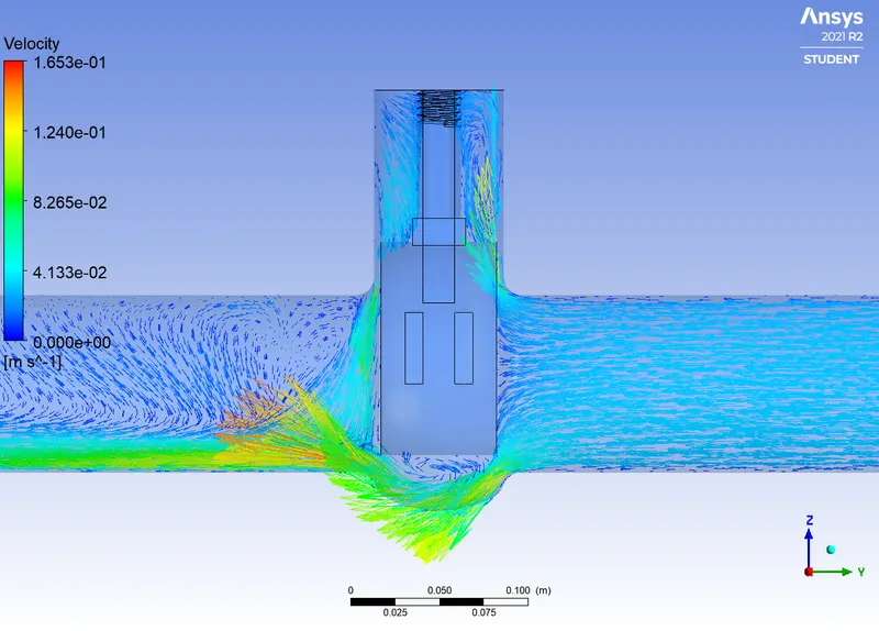
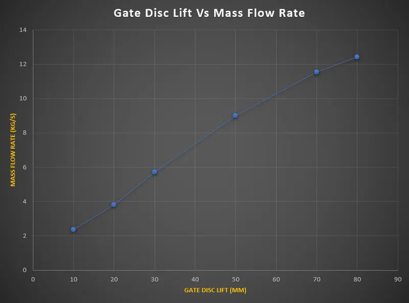
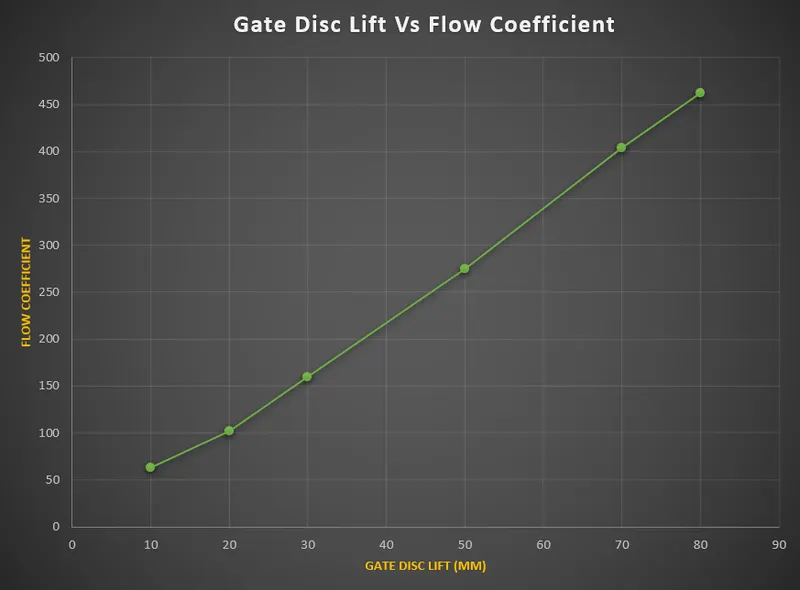
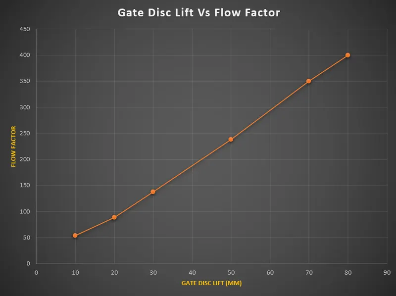
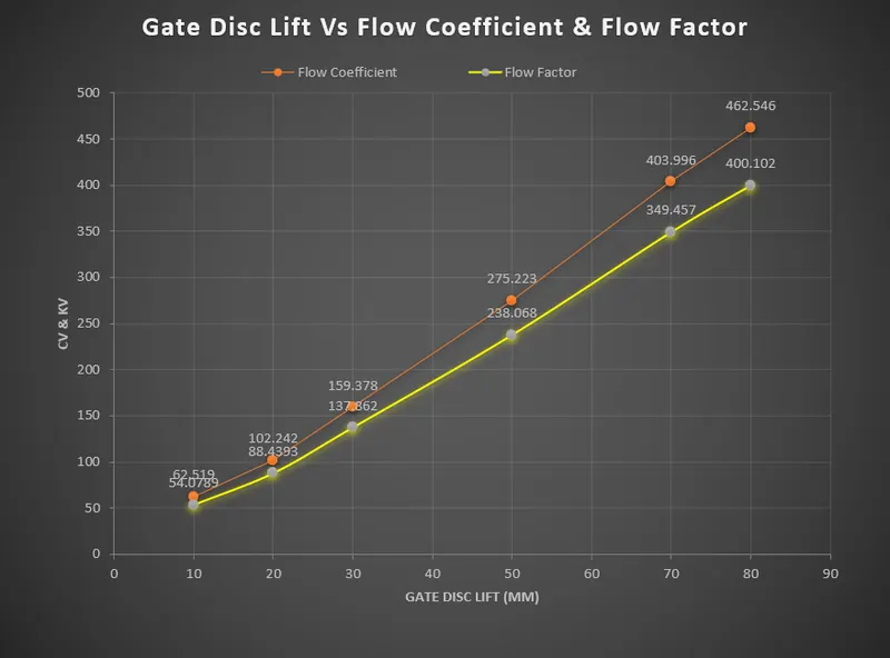
From the above results, we clearly see that the mass flow rate increases with the gate disc lift or opening. The same thing happens with the flow coefficient and the flow factor as the mass flow rate increases. Broadly, the mass flow rate, the flow coefficient and the flow factor vary linearly with the gate disc opening.
Conclusion
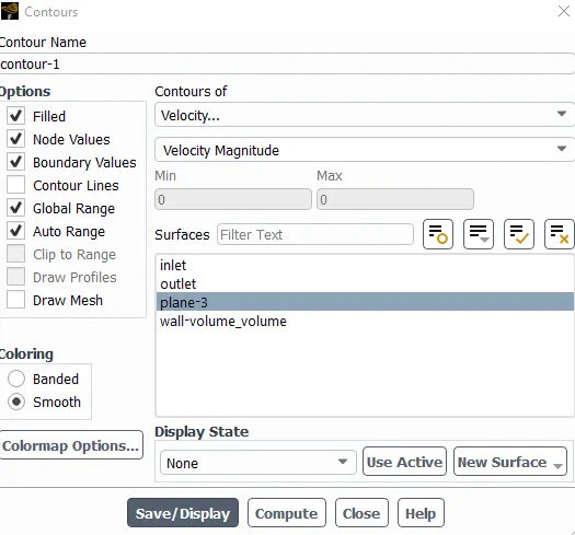
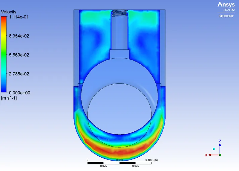
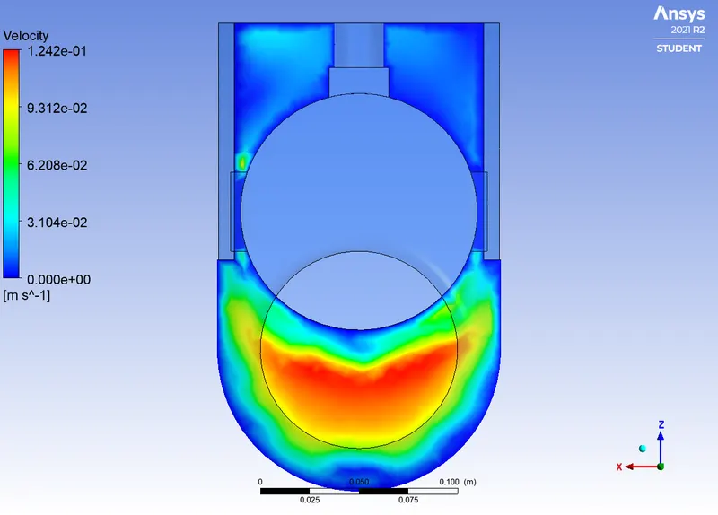
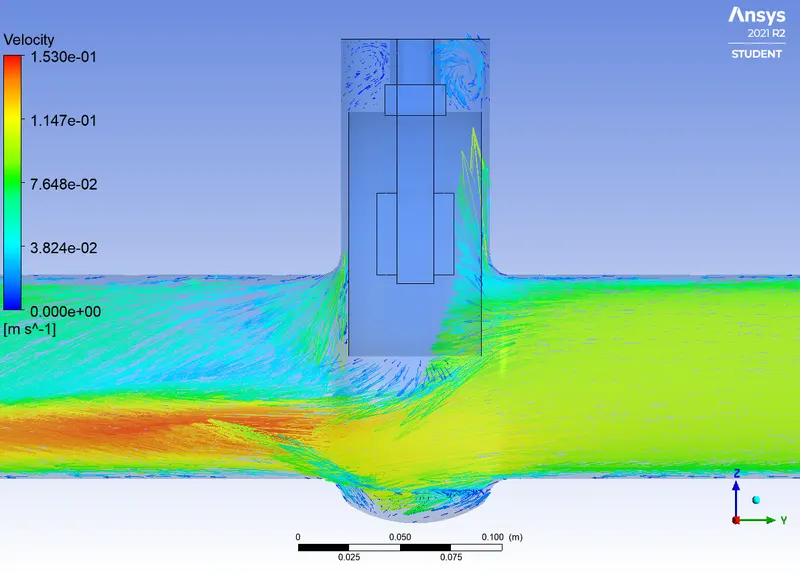
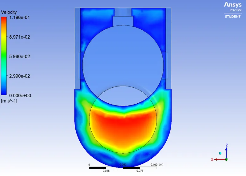
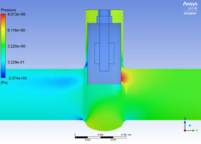
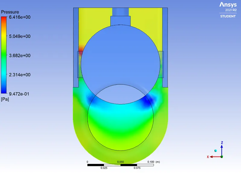
Finally, the parametric study is performed on the gate valve varying the gate disc opening from 10% to 80%. The mass flow rate, the flow coefficient and the flow factor are calculated and plotted. From the results we conclude that the velocity keeps increasing as the gate disc opening or lift increases. As for the pressure, it decreases from inlet where it is high to the outlet where it becomes 0. As the gate disc opening increases from 10% to 80%, there is an incrementation in Mass flow rate, flow coefficient and flow factor.
In the above results and graphs, one can notice that the design points corresponding to 40 mm and 60 mm are not considered; this is because the obtained results are not accurate. The reason behind this is the bug from Ansys Student version.
References: