LINEAR CONVECTION FOR VARYING THE NUMBER OF NODES

AIM: To determine the numerical solution to the one-dimensional Linear Convection equation.

PROBLEM STATEMENT:

The domain length is assumed to be L = 1m. The initial velocity profile is a step function. It is equal to 32 m/s between x = 0.1 and 0.3 and 1 m/s everywhere else. The first-order forward differencing is to be used for the time derivative and the first-order backward/rearward differencing is to be used for the space term. The constant convection coefficient is, c = 1m/s. The time step, dt = 0.01 and the simulation time, t = 0.4seconds. The simulation has to be performed for the number of nodes, n = 20, 40, 80 and 160.

OBJECTIVES:

The overall goal is to learn how to solve real world problems including PDEs, by implementing different discretization methods; and here, it’s about the linear convection problem. Thus, in this work, following points are to be achieved:

• finding the numerical solution to the one-dimensional Linear Convection equation,
• Simulating the result for different number of nodes as listed in the problem statement.
• Understand the phenomena of numerical diffusion and instability and how they relate to the courant number as well as the accuracy of the solution.

EQUATIONS USED:

• `(∂u)/(∂t)+c (∂u)/(∂x)=0`(1) This is the 1-Dimensional Linear Convection Equation where c is the constant convection coefficient and u is the velocity.
• `(du)/dt= (u(t+dt)-u(t))/dt`This is the first-order forward differencing formula applied to the velocity time derivative.
• `(du)/dx= (u(x)-u(x-dx))/dx`This is the first-order backward/rearward differencing formula applied to the velocity space derivative.
• `u_i^(n+1)=u_i^n-c.dt/dx.[u_i^n-u_(i-1)^n]`. The convection equation after discretization.

Theory:

1 D Linear convection equation: It is a hyperbolic equation and the most accessible equation in CFD.

It is obtained by keeping only accumulation and convection terms for x component from Navier Stokes equation. As it can be seen in the equations section, the coefficient of the first derivative is a constant hence the equation becomes linear.

OVERVIEW:

Programming language used: MATLAB

Loop used: for loop

Program function: “convection_func”

%this function is to calculate  the number of grids and the value of
%velocity
function [x,u_old] = convection_func(L,n,x_start,x_stop,time_march,c,dt,k)

x = linspace(0,L,n); %Defining grid points
dx= x(2)-x(1);
n_start = ((x_start)/dx)+1; %Calculation of the starting node position
n_stop = ((x_stop)/dx)+1;   %Calculation of the node position where velocity change stops
u = ones(1,n);
u(n_start:n_stop)=2;
u_old = u;
u_initial = u; % This is to show the initial profile of velocity
for i = 1:time_march
    for j = 2:n
        u(j) = u_old(j) - (c*(dt/dx)*(u_old(j)-u_old(j-1)));
    end
    u_old = u;
    figure(k)
    plot(x,u_initial,'r','linewidth',3)
    hold on
    plot(x,u,'b')
    axis([-0.1 1.5  0 5])
    xlabel('Dommain length')
    ylabel('Velocity')
    
end


end

Stepwise Explanation of the program function:

• The function takes 8 variables as inputs and returns two output values.
• The grid points are defined using “linspace” command. Then the space marching, the starting and ending nodes are computed.
• The velocity is defined and the “ones” command is used to assign the values to the velocity variable u. After that the value 2 is assigned to the velocity variable u for x>=0.1 and x<=0.3.
• After that, the time derivative and space derivative are computed in two “for loop”. The first loop is for the time and the second one is for space.
• The time derivative is computed using the first-order forward differencing and the space derivative is computed using the first order backward differencing.
• Finally comes the plotting part. The initial velocity profile is plotted against the grid points and the change in velocity is also plotted against the grid points.

Program:

clear all
close all
clc

%Inputs for linear convection problem

L = 1;
n = [20 40 80 160];
c = 1;
t = 0.4;
dt = 1e-2;
x_start = 0.1;
x_stop = 0.3;
time_march = t/dt; %This is the number of time marching steps

for k = 1:length(n)
    
   [X,U] =  convection_func(L,n(k),x_start,x_stop,time_march,c,dt,k); 
end

Stepwise explanation of the program:

• The first block is about the freeing of the memory using “clear all”, “close all” and “clc” commands.
• The second block is about the definition of the input variables present in the problem statement.
• The third and last block is about the calling of the program function. This is done in a “for loop”. This loop runs along the length n which is 4; because n is an array containing 4 numbers for grid points.

Results and discussion:

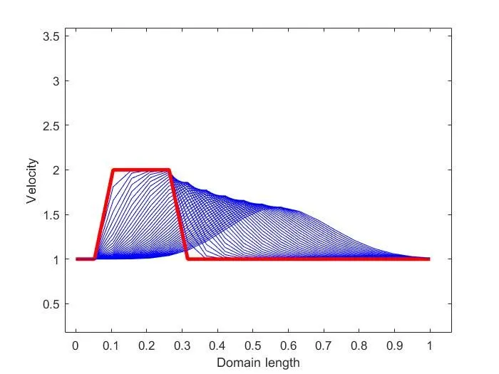
• n = 20

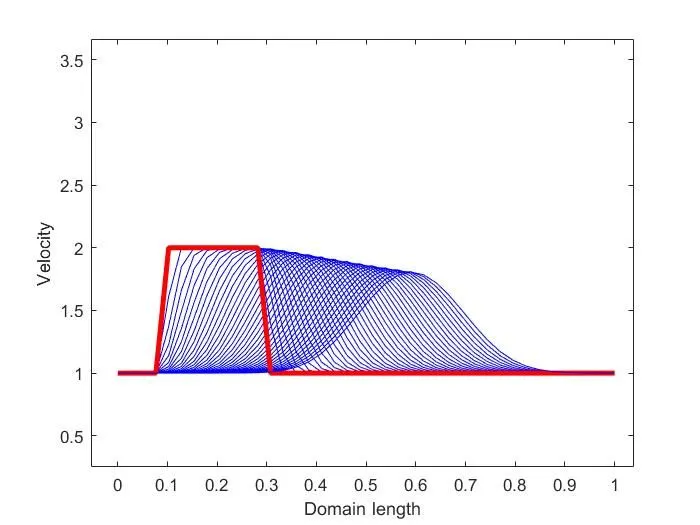
• n = 40

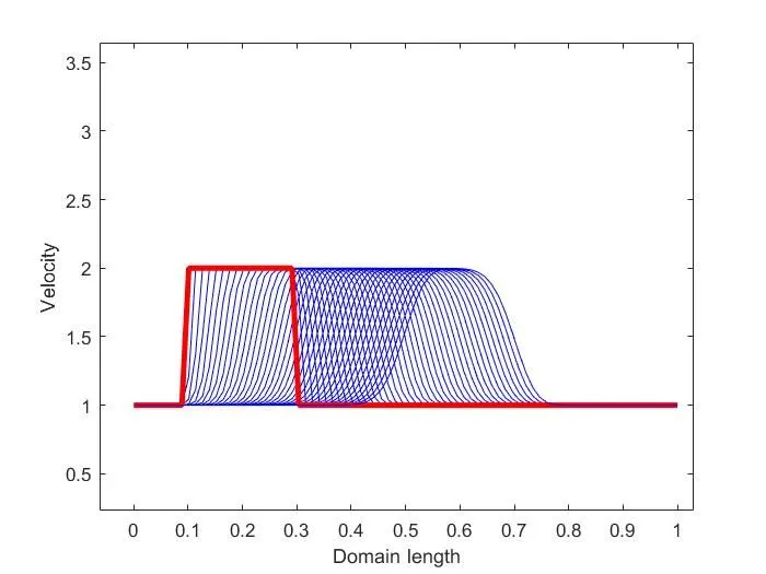
• n = 80

• n = 160

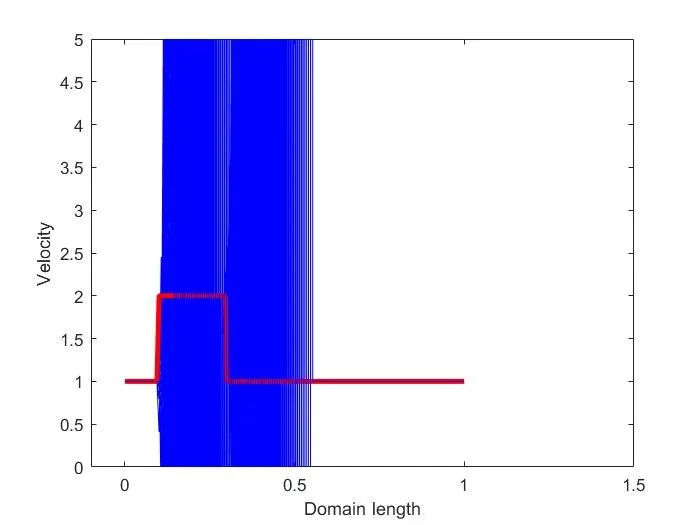
As it can be seen mainly on the fourth graph, the graph blows up this is the effect of numerical diffusion.

In fact, discretizing the equation (1) using the finite difference methods listed above and applying Taylor series to expand each term, a new concept called numerical diffusion is introduced. This concept is expressed by

`μ_num=c (∆x)/2(1-c( ∆t)/(∆x))`.

In the above equation, the term on RHS is at the origin of the instability of the solution hence it needs to be positive. This condition is equivalent to the equation below:

`c (∆x)/2 (1-c (∆t)/(∆x))≥0 → C≤1` Where `C=c (∆t)/(∆x)`is the Courant number.

This equation states the CFL condition which is also the stability condition for the equation (1). The solution will become instable as long as this solution is not respected.

Now, coming back to our work, we can notice through the different plots that from the first plot (n=20) to the third plot (n=80), the dispersion in the curve is reducing and the Courant number is C=0.19, 0.39, 0.787 and 1.587 for n=20,40, and 80 respectively. It means that, the solution is getting more and more stable and the accuracy is also improved since the Courant number is approaching to 1. But in the last case (n=160), the Courant number is equal to 1.587 which means that C > 1. As the consequence, the solution blows up.