Rayleigh Taylor Instability
Aim: The main purpose of this work is to understand the concept of Rayleigh Taylor Instability and perform its simulation using Ansys Fluent.
Objectives:
The objectives pursued throughout this work are multiple:
- Understand and explain some practical CFD models that have been based on the mathematical analysis of Rayleigh Taylor waves
- Perform the grid independency test apart from the base case simulation of the Rayleigh Taylor Instability and explain the effect of mesh size on the simulation.
- Run another simulation with water and a user-defined material for refined mesh
- Define and calculate the Atwood Number for the above cases.
Theory:
The Rayleigh-Taylor instability is the instability that occurs at the interface of two fluids of different densities; as according to density, we have heavier fluid like mercury and lighter fluid like water. This phenomenon is due to the thrust of the heavier fluid on the lighter fluid. An example of this, is the water suspended in oil.
The mathematical analysis of the Rayleigh-Taylor instability has enabled the development of different practical CFD models which are nowadays used across many industries. The types of instabilities and Some of these models are outlined below:
Ritchmyer-Meshkov instability
The Richtmyer-Meshkov instability arises when a shock wave interacts with an interface separating two different fluids. It combines compressible phenomena such as shock interaction and refraction with hydrodynamic instability, including nonlinear growth and subsequent transition to turbulence, across a wide range of Mach numbers.
Kelvin-Helmholtz Instability
The instability of Kelvin-Helmholtz is a wave motion in fluid dynamics that forms when two fluids thermally stable are superimposed and move at different velocities at their contact surface. This instability plays a n important role in many geophysical situations: in the dynamics of the atmosphere and the oceans, in the behaviour of plasmas.
Plateau-Rayleigh Instability
The instability of Plateau-Rayleigh often called Rayleigh explains why and how a fluid that falls split into packets smaller with the same volume but a lower surface. It is related to Rayleigh-Taylor and is part of the fluid dynamic branch concerned with the separation of fluid flow. The dominant phenomenon in Plateau-Rayleigh instability is the tendency of fluids to minimize their surface area due to surface tension.
Practical CFD models
Smoothed-Particle Hydrodynamics (SPH)
Developed by Gingold and Monaghan and Lucy in 1977, SPH is a computational method which is used to simulate the mechanics of continuum media such as solid mechanics and fluid flows. Initially, this model was developed for astrophysical problems. It is used in many fields such as astrophysics, ballistics, volcanology and oceanography. SPH is a meshfree method, which makes it ideally suited to simulate problems dominated by complex boundary dynamics like free surface flows or large boundary displacement. The computational cost of SPH simulations per number of particles is significantly less than the cost of grid-based simulations per number of cells when the metric of interest is related to fluid density.
Single-Fluid model
A typical approach used for the analysis of two-phase flows is a mixture model, i.e. the individual fluid phases are assumed to behave as a flowing mixture described in terms of the mixture properties. The applied single-fluid model is a five-equation model consisting of the mass, momentum and energy equations for a vapor/liquid mixture, and two equations describing the formation and growth of the liquid phase.
Two-Fluid model
In the two-fluid model, separate sets of the governing equation for the vapor and liquid phases have been used. The interaction between the droplets and the heat exchange between the liquid phase and the solid boundary are not modelled here as well. Additionally, the velocity slip between vapor and the liquid phase is in this model taken into account.
Turbulence model
Turbulence models are needed to predict the average mixing behaviour in flows that are on average one or two-dimensional. The approach to the construction of tile turbulence model is guided by the experimental behaviour. The equations governing turbulent flows can only be solved directly for simple cases of flow. For most real-life turbulent flows, CFD simulation use turbulent models to predict the evolution of turbulence. These turbulence models are simplified constitutive equations that predict the statistical evolution of turbulent flows.
Now, the following part is about the simulation of Rayleigh-Taylor Instability using Ansys Fluent. The simulation is done for two cases dealing with mesh refinement and another case in which water is used with a user-defined material of density 400kgm3 and viscosity of 0.001 kg/m.s.
Geometry
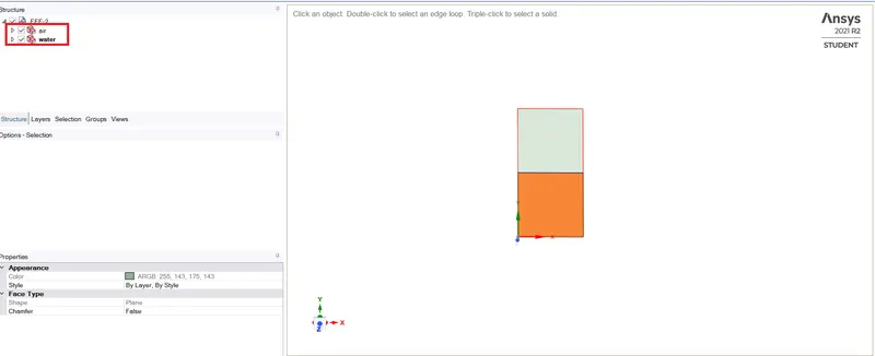
Two squares of 20 mm size are created in SpaceClaim. The top square is assigned the water surface and the bottom one is assigned the air surface. In order to create a conformal mesh in mesh module, the topology share is done enabling these two surfaces to share information’s with each other easily.
Meshing
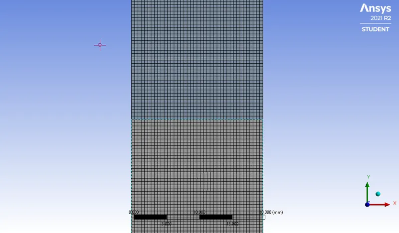
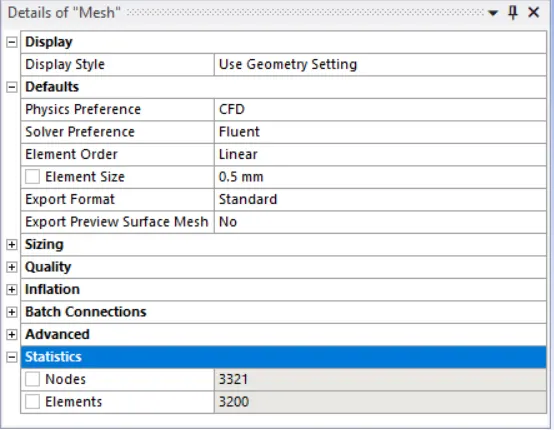
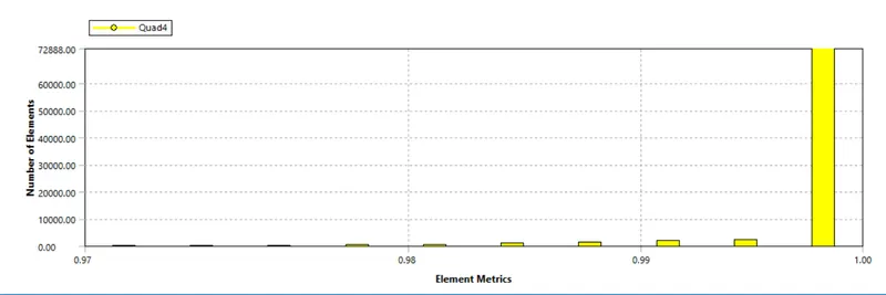
Once in the mesh module, a base mesh of 0.5 mm size is crated for base case simulation.
Mesh Refinement:
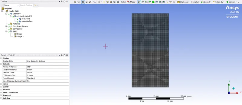
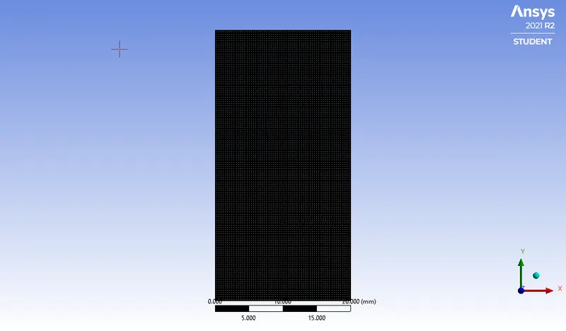
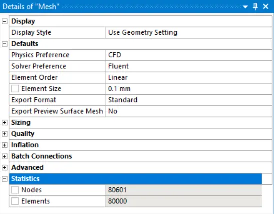
Two other cases are set up with more refined mesh of size 0.3mm and 0.1mm respectively.
Apart from these two cases, one more simulation is run where water and a user-defined material are used as state above.
Case 1: Mesh size is 0.3 mm
Case 2: Mesh size is 0.1mm
Setting up the case
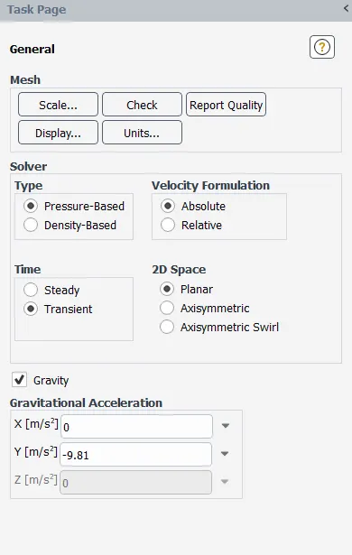
Transient simulation is done with a pressure-based solver. The gravity is enabled in negative y-direction according to the Rayleigh-Taylor instability definition. The simulation is done as laminar and material used are water and air.
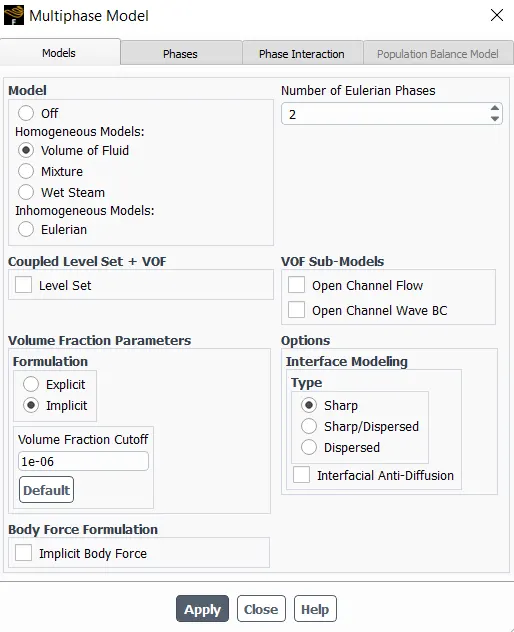
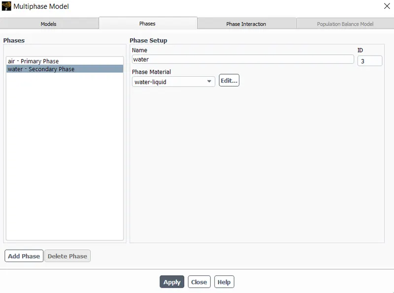
The multiphase is used along with volume of fluid model and implicit formulation where the primary phase represents air and the secondary phase represents water.
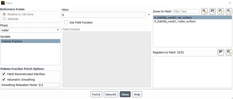
After that, standard initialization is done and the computational domain is marked using patch option as shown on the snippets below to distinguish each phase. Then, the calculations are run.
Output
Base Case, Mesh Size 0.5mm
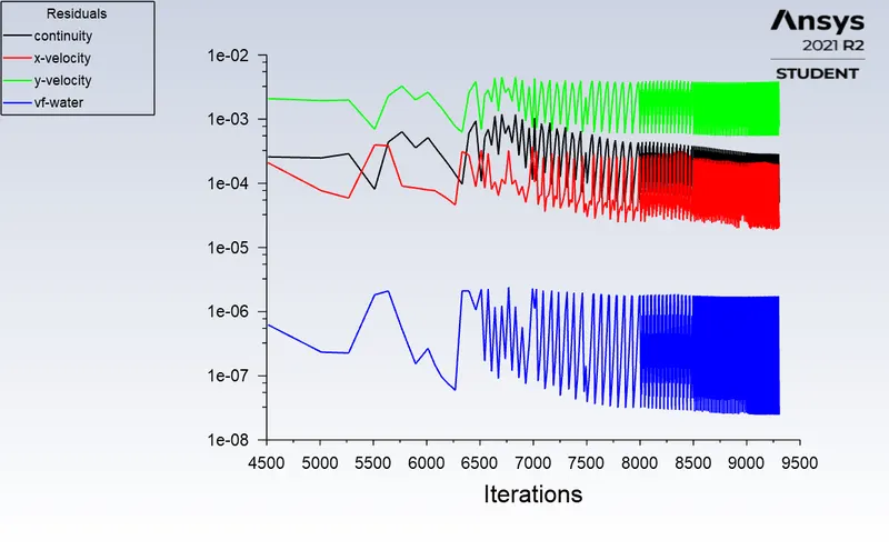
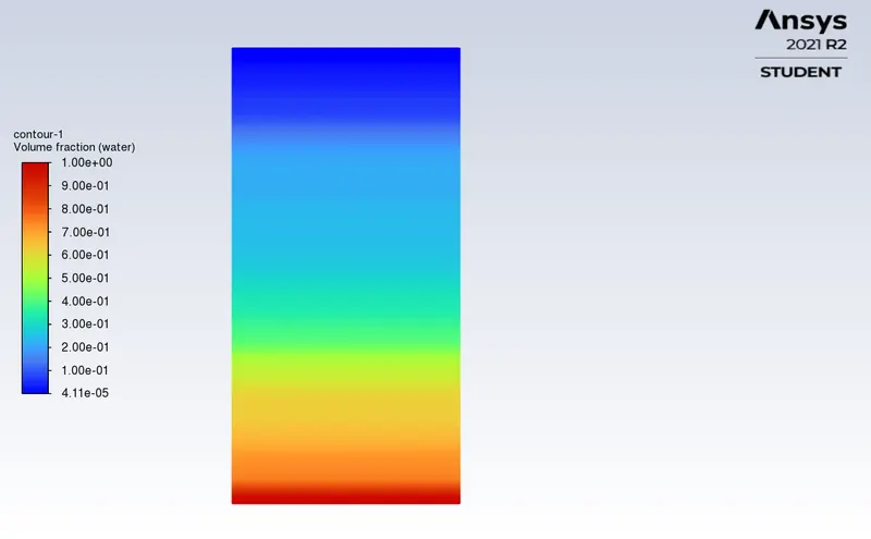
Click here for Base case animation
Refinement Cases
Case 1: Mesh size is 0.3 mm
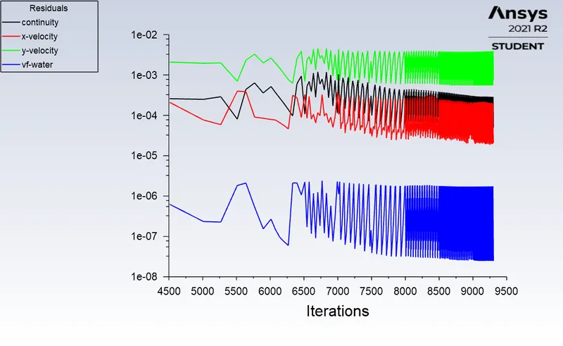
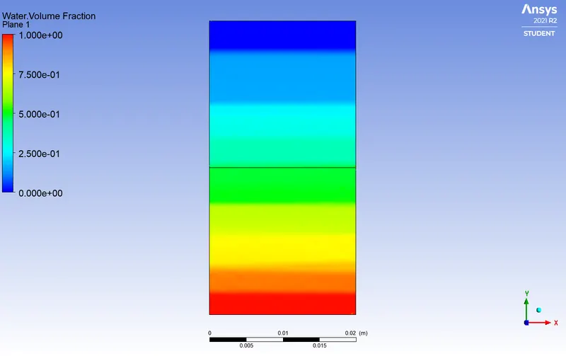
Click here to view the case 1 animation
Case 2: Mesh size is 0.1mm
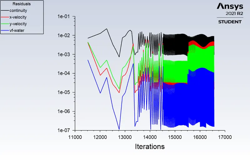
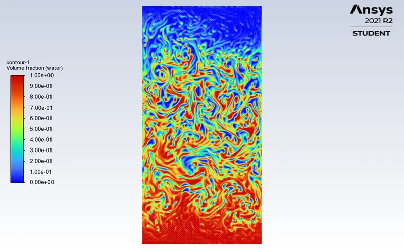
click here for animation case2
Case 3: Mesh size is 0.1mm with water and user-defined material
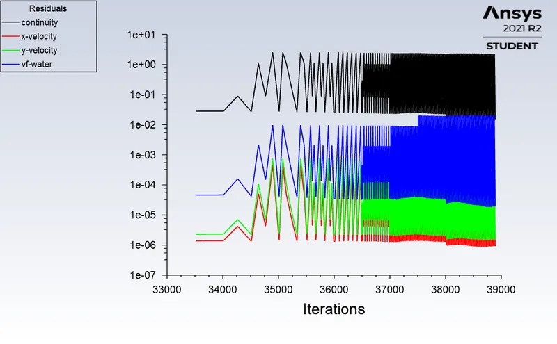
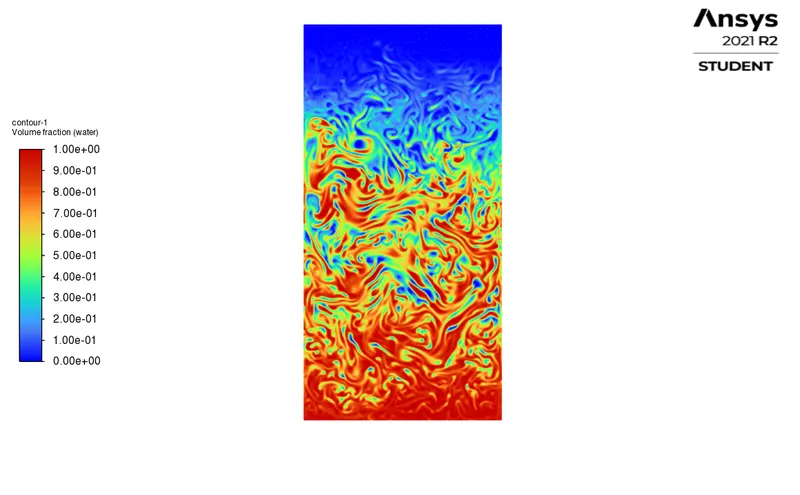
Click here for animation case3
Atwood Number
The two-dimensional Rayleigh-Taylor instability described by a configuration such as average velocity U (x, z) =W (x, z) =0, and the gravitational field is g= -gŷ with an interface separating fluids of two different densities. The Atwood Number (A) is a dimensionless number used in fluid mechanics to characterize Rayleigh-Taylor instability also termed as hydrodynamic instability of fluids with density stratification. It is a density ratio and is defined as follows:
`A=(ρ_1-ρ_2)/(ρ_1+ρ_2 )`
Where ρ1 and ρ2 are density of heavy fluid and density of light fluid respectively.
Calculation of Atwood Number
Case1:
Heavier fluid (Water), density (ρ1) = 998.2kg/m3
Lighter fluid (Air), density (ρ2) = 1.225kg/m3
This implies that the Atwood Number (A) = 0.998
Case2:
Heavier fluid (Water), density (ρ1) = 998.2kg/m3
Lighter fluid (User-defined fluid), density (ρ2) = 400kg/m3
This implies that the Atwood Number (A) = 0.428
In Rayleigh-Taylor instability analysis, the Atwood Number is an important parameter. Indeed, for Atwood Number close to zero, the Rayleigh-Taylor instability flows behave as asymmetric finger of fluid; and for Atwood Number close to 1, the lighter fluid at the bottom forms larger bubble-like plume.
According to the calculations done above, the Atwood Number is much close to 1 in the first case and through the simulation results one can see with the initial configuration (heavier fluid (water) poured upon the lighter fluid (air) with air subjected to gravity) that the air-bubble-like plumes are formed. These air-bubbles travel upwards in the form of waves among which some got trapped at the lower region just at the beginning stages. By the convergence of the solution, the trapped remaining trapped air-bubbles have moved upward and the two phases are now separated leaving some diffusivity at the middle or at the interface of the two fluids.
Effect of Atwood Number on the instability behaviour
In linear stability analysis, it is found that the least disturbance of the interface is amplified exponentially with rate:
`e^γt ,with γ=√Agα , where , α :is the spatial wave number and A is the Atwo od Number`
Throughou9t the two cases, we can see that the growth of bubble thickness is suppressed at small Atwood Number (case 2) whereas it is enhanced at large Atwood Number (case 1). This can be observed through the different animation.
References
- https://fr.wikipedia.org/wiki/Instabilit%C3%A9_de_Kelvin-Helmholtz
- https://fr.wikipedia.org/wiki/Instabilit%C3%A9_de_Plateau-Rayleigh
- https://skly.in/student-projects/rayleigh-taylor-instability-challenge-98
- https://aip.scitation.org/doi/abs/10.1063/5.0071437