SOLVING THE 2D STEADY STATE AND TRANSIENT HEAT CONDUCTION EQUATION USING MATLAB

AIM: To perform steady state analysis and transient analysis

OBJECTIVES:

• To understand how to use iterative solvers to solve a problem.
• Learn how to implement methods such as:
• Jacobi method
• Gauss-Seidel method
• Successive over-relaxation.
• The explicit and implicit approaches.

Introduction:

Most of the physical systems have two types of solutions that are the steady state solution and transient solution. Thus, it becomes necessary to perform steady state analysis and transient analysis to properly design and evaluate systems.

PROBLEM STATEMENT:

1. Steady state analysis & Transient State Analysis

Solve the 2D heat conduction equation by using the point iterative techniques that were taught in the class. The Boundary conditions for the problem are as follows;

Top Boundary = 600 K

Bottom Boundary = 900 K

Left Boundary = 400 K

Right Boundary = 800 K

You will implement the following methods for solving implicit equations.

1. Jacobi
2. Gauss-seidel
3. Successive over-relaxation

Your absolute error criteria is 1e-4

2. You will write code for both implicit and explicit schemes (This is for the Transient Analysis only)
3. Write a detailed explanation for your results

EQUATIONS USED:

The main equations used in this problem are:

• `(∂^2 T)/(∂x^2) +(∂^2 T)/(∂y^2) =0`(1) This is the 2D steady state form of the heat conduction equation.
• `(DT)/(Dt)+α((∂^2 T)/(∂x^2) +(∂^2 T)/(∂y^2) )=0`(2) This is the 2D transient heat conduction equation.

Theory:

Steady state solution is can be seen as the solution that does not converge to zero as the time approaches infinity. Unlike steady state solution, the transient solution converges to zero as time approaches infinity.

Since the temperature is the solution of the equation under studies, two analyses will be done: the steady state thermal analysis and transient thermal analysis.

1. STEADY STATE ANALYSIS

In this part, the equation 1 is used.

This equation is discretized using central differencing for 2nd order derivative.

• `(D^2 T)/(Dx^2) =(T_(i+1,j)-2*T_(i,j)+T_(i-1,j))/(∆x^2)`
• `(D^2 T)/(Dy^2) =(T_(i,j+1)-2*T_(i,j)+T_(i,j-1))/(∆y^2)`

By replacing these expressions in the equation 1, we get a linear equation as follows:

`(T_L-2*T_P+T_R)/(∆x^2) +(T_T-2*T_P+T_B)/(∆y^2) =0`

This leads to:

`T_P ((∆x^2+∆y^2)/(∆x^2*∆y^2 ))=RHS`

If `k= ((∆x^2+∆y^2)/(∆x^2*∆y^2 ))` , then we finally have:

`T_P= 1/k [((T_L+T_R)/(∆x^2 ))+((T_T+T_B)/(∆y^2) )]`

This expression is used to compute the temperature using different methods as listed above.

Program: For steady state analysis

%This program is to solve the two Dimensional steady state Heat conduction equation

clear all
close all
clc


%Definition of the inputs anmd initial conditions

L = 1;%Domain length
nx = 11; %input('1,2,3')
ny = nx;

x = linspace(0,L,nx);
y = linspace(0,L,ny);
dx = x(2)-x(1);
dy = y(2)-y(1);


error = 9e9;
tol = 1e-4;

%Boundary condition
T_T = 600;
T_B = 900;
T_L = 400;
T_R = 800;
%defining the Temperature matrix
T = 298*ones(nx,ny);
T(1,:) = T_B;
T(end,:) = T_T;
T(:,1) = T_L;
T(:,end) = T_R;

%The commands below are for the refinement of the edges of matrix T
T(1,1) =(T_B+T_L)/2;
T(end,1) = (T_L+T_T)/2;
T(1,end) = (T_B+T_R)/2;
T(end,end) = (T_T+T_R)/2;

% Definition of relaxation factor
omega = 0.8;

%Let's create a copy of old values of T
Told = T;
[X,Y] = meshgrid(x,y);

%Chosing the iterative solver
iterative_solver = input('1 Jacobi 2 Gauss Seidel 3 SOR  nEnter the option corresponding to the type of solver to be used: n=');
 k = 2/(dx)^2 + 2/(dy)^2;
% k1 = 0.5*(dy^2/(dy^2+dx^2));
% k2 = 0.5*(dx^2/(dy^2+dx^2));

tic
if iterative_solver == 1
    jacobi_iter =1;
    while(error > tol)
        for i =2:nx-1
            for j =2:ny-1
                term1 = (Told(i-1,j)+Told(i+1,j))/(k*((dx)^2));
                term2 = (Told(i,j-1)+Told(i,j+1))/(k*((dy)^2));
                T(i,j) = term1+term2;
            end
        end
        error = max(max(abs(Told-T)));
        Told = T;
        jacobi_iter = jacobi_iter + 1;
        
        %Plotting the contour
        figure(1)
        [A,B] = contourf(X,Y,T);
        colorbar
        colormap(jet)
        clabel(A,B)
        xlabel('X axis');
        ylabel('Y axis');
        title_text = sprintf('Steady-Staten Jacobi Iteration Number= %d',jacobi_iter);
        
        title(title_text);
        pause(0.03)
        
    end
        
    
    
end


if iterative_solver == 2
    gs_iter = 2;
    while(error > tol)
        for i =2:nx-1
            for j =2:ny-1
                term1 = (T(i-1,j)+Told(i+1,j))/(k*((dx)^2));
                term2 = (T(i,j-1)+Told(i,j+1))/(k*((dy)^2));
                T(i,j) = term1+term2;
            end
        end
        error = max(max(abs(Told-T)));
        Told = T;
        gs_iter = gs_iter + 1;
        
        %Plotting the contour
        figure(1)
        [A,B] = contourf(X,Y,T);
        colorbar
        colormap(jet)
        clabel(A,B)
        title_text = sprintf('Steady-Staten Gauss Seidel Iteration Number= %d',gs_iter);
        xlabel('X axis')
        ylabel('Y axis');
        title(title_text);
        pause(0.03)
        
    end
    
    
end

if iterative_solver == 3
    sor_iter = 3;
    while(error > tol)
        for i =2:nx-1
            for j =2:ny-1
                term1 = (Told(i-1,j)+Told(i+1,j))/(k*((dx)^2));
                term2 = (Told(i,j-1)+Told(i,j+1))/(k*((dy)^2));
                T(i,j) = (1-omega)*(Told(i,j)) + omega*(term1+term2);
            end
        end
        error = max(max(abs(Told-T)));
        Told = T;
        sor_iter = sor_iter + 1;
        
        %Plotting the contour
        figure(1)
        [A,B] = contourf(X,Y,T);
        colorbar
        colormap(jet)
        clabel(A,B)
        title_text = sprintf('Steady-Staten SOR Iteration Number= %d',sor_iter);
        xlabel('X axis')
        ylabel('Y axis');
        title(title_text);
        pause(0.03)
        
    end
    
    
end


Time_taken = toc

Stepwise explanation of the program:

• The input variables are defined after freeing the memory.
• The boundary conditions given in the program statement are defined. Then, the edges are refined using the average value.
• A copy of temperature matrix is created.
• Then comes the main part. It is constituted of three subparts; each one contained within a “if condition”.
• There are in total three “if condition” statements for choosing the iterative solver; each one corresponding to Jacobi method, Gauss Seidel and successive over-relaxation.
• In each “if condition” block, there is a “while condition” which is satisfies the error criteria and contains two space loops. After these loops, the error is computed, the temperature values are updated and plotting is done.
• These three blocks are contained in a time measuring commands that are “tic” and “toc” letting us to know the running time taken by the program.

Output:

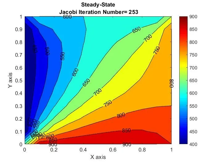
Time_taken = 60.4392

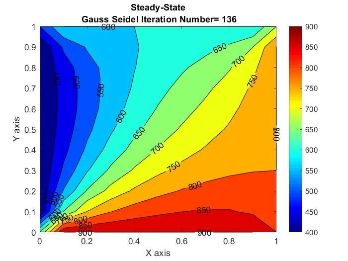
Time_taken = 30.9219

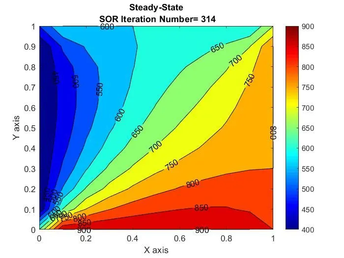
Time_taken = 71.5655

1. TRANSIENT ANALYSIS

In this analysis, two approaches will be used: the explicit approach and the implicit approach. The equation used here is the equation 2:

`(DT)/(Dt)+α((∂^2 T)/(∂x^2) +(∂^2 T)/(∂y^2) )=0`

For the discretization of this equation, the space derivatives are discretized using the previous formulae and the time derivative is discretized using the formula below:

`(DT)/(Dt)=(T^(n+1)_(i,j)-T^n_(i,j))/(∆t)`

As a result, the following equation is obtained:

`T_P^(n+1)= T_P^n+α∆t[((T_L-2*T_P+T_R)/(∆x^2) +(T_T-2*T_P+T_B)/(∆y^2) )]^(n or n+1) (3)`

Where n and n+1 are two consecutive time steps and `k1=α (∆t)/(∆x^2) ; k2=α( ∆t)/(∆y^2)`

Explicit approach is a scheme in which the Partial differential equation is discretized in such a way that there is only one unknown corresponding to an advance time step (n+1). Thus, the solution is evaluated in terms of known quantities.

In the equation 3, when the time step on the right-hand side is chosen to be n, the method to be implemented is called explicit method or explicit approach.

Thus, the new equation obtained is as follows:

`T_P^(n+1)= T_P^n+k1[T_L-2*T_P+T_R ]^n+k2[T_T-2*T_P+T_B ]^n`

Program:

%This program is to solve the two Dimensional Transient state Heat
%conduction equation using explicit method
clear all
close all
clc


%Inputs
%Definition of the inputs anmd initial conditions

L = 1;%Domain length
%Space marching
nx = 10; %input('1,2,3')
ny = nx;
%time marchingdefinition
dt = 0.001;

%Space marching
x = linspace(0,L,nx);
y = linspace(0,L,ny);
dx = x(2)-x(1);
dy = y(2)-y(1);

%Definition of diffusivity factor alpha
alpha = 1.5;

k1 = (alpha*dt)/((dx)^2);
k2 = (alpha*dt)/((dy)^2);

% Verification of stability criteria
CFL = k1+k2; % This value should be less than 0.5 for the explicit solution

%Definition of the error criteria
error = 9e9;
tol = 1e-4;

%Boundary condition
T_T = 600;
T_B = 900;
T_L = 400;
T_R = 800;

%defining the Temperature matrix
T = 400*ones(nx,ny);
T(1,:) = T_B;
T(end,:) = T_T;
T(:,1) = T_L;
T(:,end) = T_R;

%The commands below are for the refinement of the edges of matrix T
T(1,1) =(T_B+T_L)/2;
T(end,1) = (T_L+T_T)/2;
T(1,end) = (T_B+T_R)/2;
T(end,end) = (T_T+T_R)/2;

%Let's create a copy of old values of T
Told = T;
[X,Y] = meshgrid(x,y);


tic
transient_explicit_iter =1;
for nt = 1:400
    
    for i =2:nx-1
            for j =2:ny-1
                term1 = Told(i,j);
                term2 = Told(i-1,j)-2*Told(i,j)+Told(i+1,j);
                term3 = Told(i,j-1)-2*Told(i,j)+Told(i,j+1);
                T(i,j) = term1+k1*term2+k2*term3;
            end
            
        Told = T;
        transient_explicit_iter = transient_explicit_iter + 1;
        
        %Plotting the contour
        figure(1)
        [A,B] = contourf(X,Y,T);
        colorbar
        colormap(jet)
        clabel(A,B)
        title_text = sprintf('Transient Explicitn Iteration Number= %d',transient_explicit_iter);
        xlabel('X axis')
        ylabel('Y axis');
        title(title_text);
        pause(0.003)
        
    end
    
    
end

time_taken = toc

Stepwise explanation of the program:

• The input variables are defined after freeing the memory.
• The boundary conditions given in the program statement are defined. Then, the edges are refined using the average value.
• A copy of temperature matrix is created.
• Then comes the main part. It is constituted of a time loop in which two space loops are defined since the problem is a 2 dimensional one. The temperature values are updated and plotting is done after the space loops.
• The Jacobi method is used here for the iterations and the time loop is contained in a time measuring commands that are “tic” and “toc” letting us to know the running time taken by the program.

Output:

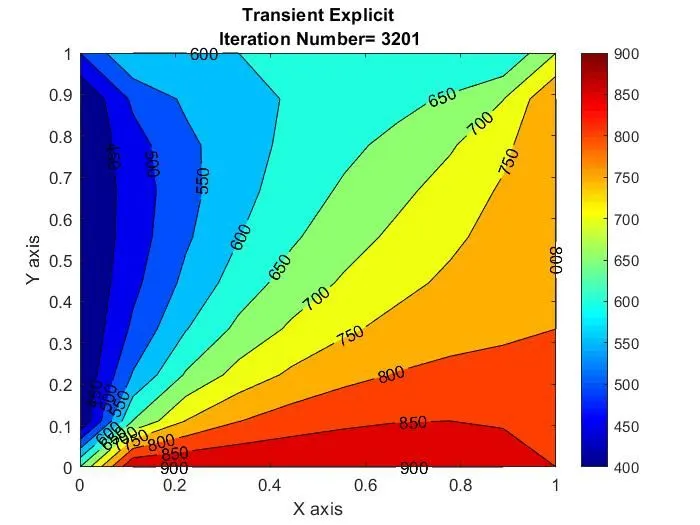
Time_taken = 928.1203

Implicit approach in contrast, is a scheme in which, the partial differential equation is discretized in such a way that the number of unknown variables is more than one. Thus, the solution will be evaluated in terms of unknown quantities, all at the new time step (n+1).

In the equation 3, when the time step on the right-hand side is chosen to be n+1, the method to be implemented is called implicit method or implicit approach.

Thus, the new equation obtained is as follows:

`T_P^(n+1)=1/(1+2k1+2k2) [T_P^n+k1[T_L+T_R ]^(n+1)+k2[T_T+T_B ]^(n+1) ]`

Program:

%This program is to solve the two Dimensional Transient state Heat
%conduction equation using implicit method
clear all
close all
clc


%Inputs
%Definition of the inputs anmd initial conditions

L = 1;%Domain length
%Space marching
nx = 10; %input('1,2,3')
ny = nx;
%time marchingdefinition
dt = 0.001;

%Space marching
x = linspace(0,L,nx);
y = linspace(0,L,ny);
dx = x(2)-x(1);
dy = y(2)-y(1);

%Definition of diffusivity factor alpha
alpha = 1.5;

k1 = (alpha*dt)/((dx)^2);
k2 = (alpha*dt)/((dy)^2);

% Verification of stability criteria
CFL = k1+k2; % This value should be less than 0.5 for the explicit solution
omega = 1.1;
%Definition of the error criteria

tol = 1e-4;

%Boundary condition
T_T = 600;
T_B = 900;
T_L = 400;
T_R = 800;

%defining the Temperature matrix
T = 298*ones(nx,ny);
T(1,:) = T_B;
T(end,:) = T_T;
T(:,1) = T_L;
T(:,end) = T_R;

%The commands below are for the refinement of the edges of matrix T
T(1,1) =(T_B+T_L)/2;
T(end,1) = (T_L+T_T)/2;
T(1,end) = (T_B+T_R)/2;
T(end,end) = (T_T+T_R)/2;

%Let's create a copy of old values of T
Told = T;
[X,Y] = meshgrid(x,y);
T_prev_dt = Told;

iterative_solver = input('1 Jacobi 2 Gauss Seidel 3 SOR  nEnter the option corresponding to the type of solver to be used: n=');
tic
if iterative_solver == 1
transient_implicit_iter =1;
for nt = 1:400
    error = 9e9;

    while(error > tol)
        for i =2:nx-1
            for j =2:ny-1
                term1 = 1/(1+2*k1+2*k2);
                term2 = k1*term1;
                term3 = k2*term1;
                H = Told(i-1,j)+Told(i+1,j);
                V = Told(i,j-1)+Told(i,j+1);
                T(i,j) = (T_prev_dt(i,j)*term1)+(H*term2)+(V*term3);
            end
        end
        error = max(max(abs(Told-T)));
        Told = T;
        transient_implicit_iter = transient_implicit_iter + 1;
        
        
        
    end
    
    T_prev_dt = T;
    %Plotting the contour
        figure(1)
        [A,B] = contourf(X,Y,T);
        colorbar
        colormap(jet)
        clabel(A,B)
        title_text = sprintf('Transient Implicitn Jacobi Iteration Number= %d',transient_implicit_iter);
        xlabel('X axis')
        ylabel('Y axis');
        title(title_text);
        pause(0.03)
end


end





if iterative_solver == 2
transient_implicit_iter =1;
for nt = 1:1400
    
    error = 9e9;
    while(error > tol)
        for i =2:nx-1
            for j =2:ny-1
                term1 = 1/(1+2*k1+2*k2);
                term2 = k1*term1;
                term3 = k2*term1;
                H = T(i-1,j)+Told(i+1,j);
                V = T(i,j-1)+Told(i,j+1);
                T(i,j) = (T_prev_dt(i,j)*term1)+(H*term2)+(V*term3);
            end
        end
        error = max(max(abs(Told-T)));
        Told = T;
        transient_implicit_iter = transient_implicit_iter + 1;
        
        
        
        
    end
    T_prev_dt = T;
    
    %Plotting the contour
        figure(1)
        [A,B] = contourf(X,Y,T);
        colorbar
        colormap(jet)
        clabel(A,B)
        title_text = sprintf('Transient Implicitn Gauss-Seidel Iteration Number= %d',transient_implicit_iter);
        xlabel('X axis')
        ylabel('Y axis');
        title(title_text);
        pause(0.003)
end


end




if iterative_solver == 3
transient_implicit_iter =1;
for nt = 1:1400
    error = 9e9;
    while(error > tol)
        for i =2:nx-1
            for j =2:ny-1
                term1 = 1/(1+2*k1+2*k2);
                term2 = k1*term1;
                term3 = k2*term1;
                H = T(i-1,j)+Told(i+1,j);
                V = T(i,j-1)+Told(i,j+1);
                T(i,j) = (1-omega)*Told(i,j)+omega*((T_prev_dt(i,j)*term1)+(H*term2)+(V*term3));
            end
        end
        error = max(max(abs(Told-T)));
        Told = T;
        transient_implicit_iter = transient_implicit_iter + 1;
        
        
        
    end
    T_prev_dt = T;
    
    
        %Plotting the contour
        figure(1)
        [A,B] = contourf(X,Y,T);
        colorbar
        colormap(jet)
        clabel(A,B)
        title_text = sprintf('Transient Implicitn SOR Iteration Number= %d',transient_implicit_iter);
        xlabel('X axis')
        ylabel('Y axis');
        title(title_text);
        pause(0.003)
end

end
time_taken = toc

Stepwise explanation of the program:

• This program as it can be seen has the same structure as the one for the steady state analysis. The only difference is the formulae used. Thy are different as shown by the mathematical expressions derived above.

Output:

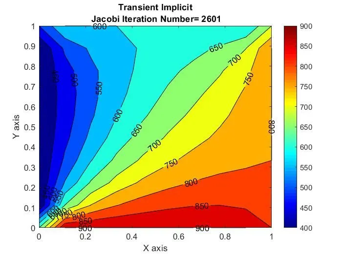
Time_taken = 104.1110

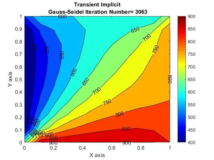
Time_taken = 355.7359

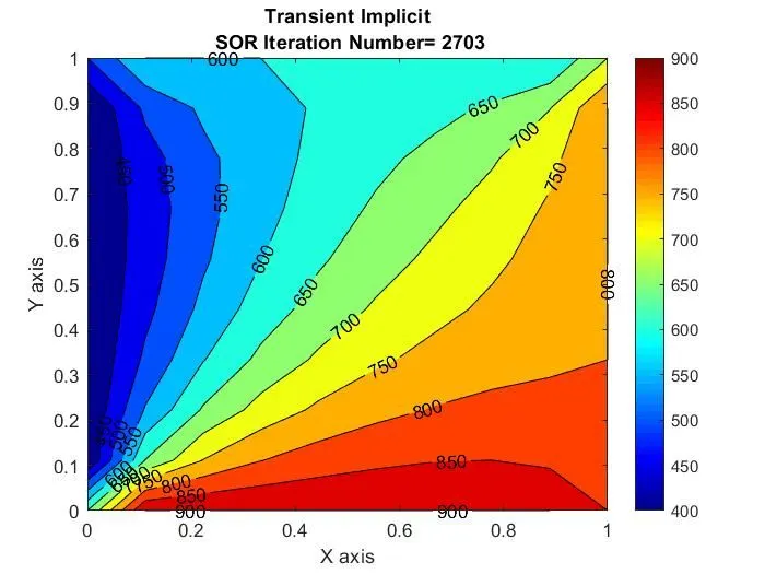
Time_taken = 337.4006

Discussion of the results:

Throughout the different outputs, we can see that the number of iterations is less in the case of steady state analysis as compared to the number of iterations in the transient analysis. As a result, the processing time taken is much more import in transient analysis as compared to steady state analysis.

Conclusion:

At the end of our work, we can say that iterative solvers are important to solve some problems. However, they require much time depending on the type of the analysis and sometimes much resources depending on the method to be implemented such as implicit method.

REFERENCES:

• https://www.researchgate.net/post/What_is_the_difference_between_implicit_and_explicit_solutions_of_the_numerical_solutions
• https://www.flow3d.com/resources/cfd-101/numerical-issues/implicit-versus-explicit-numerical-methods/