RANKINE CYCLE SIMULATOR
AIM: This project aims to create a Rankine Cycle Simulator by using MATLAB.
OBJECTIVES:
- Calculate the state points of the Rankine Cycle,
- Plot the corresponding T-s and h-s diagrams for the given set of inputs,
- Calculate the Net work output,
- Calculate work ratio.
THEORY :
Rankine cycle is the theoretical cycle on which the steam turbine works. It is an idealized cycle in which losses in each of the four components are neglected. Used to produce mechanical work, the Rankine Cycle is particularly employed to predict the work produced by a steam turbine system in a heat engine.
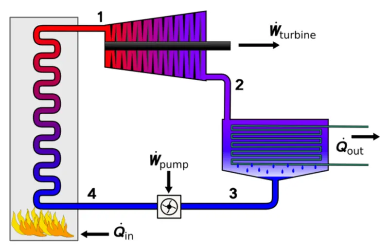
The main components forming Rankine Cycle are as follow:
- Steam generator: Boiler
It turns the fluid at room temperature and pressure to superheated vapour or steam which is a vapour whose temperature is greater than the saturation temperature corresponding to the pressure of the vapour.
Now applying steady flow energy equation to boiler, turbine, condenser and pump;
As for control volume we get in this case:
`h_f4+ Qi n= h_1`
`Qi n= h_1- h_f4`
- Steam Turbine
Here, the pressure is increased causing a drop in temperature hence the mechanical work is produced.
As for control volume we get:
`h_1= W_T+ h_2`
`Where W_T= Turbi n e w o r k`
`W_T= h_1- h_2`
- Condenser:
The condenser operates isothermally and rejects heat in the environment. The fluid state is compressed back to liquid-gas mixture that is mostly liquid called saturated-liquid.
As per such reaction, we get:
`h_2= Qout+ h_f3`
`Qout= h_2- h_f3`
- Pump
The saturated-liquid at this level is pressurized back to the pressure of the turbine by supplying the work to the system resulting in a compressed liquid.
We get:
`h_f3+ W_P= h_f4`
`Where W_P= Pump w o rk`
`W_P= h_f4- h_f3`
Efficiency of Rankine Cycle is given by:
`η_Ranki n e= (Wn et)/(Qi n) = (W_T-W_P)/(Qi n)`
The four components listed above work conjointly through four ideal processes:
- Reversible adiabatic expansion in the Turbine
- Constant-pressure transfer of heat in the condenser
- Reversible adiabatic pumping process in the feed pump
- Constant-pressure transfer of heat in the boiler
REQUIRED INPUTS:
- Turbine Inlet temperature = 400°C
- Turbine Inlet Pressure = 30 bars
- Turbine Outlet Pressure = 0.05 bars = Condenser Inlet
PROGRAM:
clear all
close all
clc

%%commands to display the different phases in Rankine cycle
fprintf('               RANKINE CYCLE SIMULATOR n');
fprintf('1-2  Reversible adiabatic expansion in the Turbine n');
fprintf('2-3  Constant-pressure transfer of heat in the condenser n');
fprintf('3-4  Reversible adiabatic pumping process in the feed pump n');
fprintf('4-1  Constant-pressure transfer of heat in the boiler n');

%%inputs
%STEP 1: Entering of independent propeerties at the starting point
p1 = input('Enter the pressure at the Turbine Inlet:'); %P1 in bar
T1 = input('Enter the Temperature at the Turbine Inlet:');%T1 in Degree Celcius
p2 = input('Enter the pressure at the Condenser Inlet:');

%STEP 2:Calculation of each state point properties
%state point 1
h1 = XSteam('h_pt',p1,T1);
s1 = XSteam('s_pt',p1,T1);

%STEP 3:state point 2
s2 = s1;
sf2 = XSteam('sL_p',p2);%entropy of saturated water
sg2 = XSteam('sV_p',p2);%entropy of saturated vapour
hf2 = XSteam('hL_p',p2);%enthalpy of saturated water
hg2 = XSteam('hV_p',p2);%enthalpy of saturated vapour
x2 = (s2-sf2)/(sg2-sf2)   %s2 = sf2 +x2*(sg2 - sf2)
h2 = hf2 +x2*(hg2 - hf2)

T2 = XSteam('T_hs',h2,s2);

%STEP 4: State point 3

T3 = T2; % The process 2-3 is isothermal
p3 = p2;%pressure at state point 3
s3 = XSteam('sL_T',T3); %entropy at state point 3
h3 = XSteam('hL_T',T3);%enthalpy at state point 3
V3 = XSteam('vL_p',p3); %specific volume

%STEP 5: state point 4

p4 = p1;
s4 = s3;
Cp4 = XSteam('Cp_ps',p4,s4);%Specific isobaric heat capacity
Cv4 = XSteam('Cv_ps',p4,s4);%specific isochoric heat capacity
gamma = Cp4/Cv4;
r= (gamma - 1)/gamma;
T4 = T3*(p4/p3)^r;


%STEP 6: calculation of other output values;

Wt = h1 - h2; %Work done at the Turbine
Wp = V3*(p1-p2)*100; %Work at the feed water pump
h4 = Wp + h3;
Wnet = Wt - Wp;
Qin = h1 - h4; % heat supplied
Qout = h1 - h3;
N_per= (Wnet/Qin)*100 ;%Efficiency of the cycle
steam_rate = 3600/(Wt - Wp); %This is to calculate the steam rate per second

%STEP7: state points 5 and 6
% These points help us in plotting respective curves
T5 = XSteam('Tsat_p',p1);
T6 = T5;
s5 = XSteam('sL_p',p1);
s6 = XSteam('sV_p',p1);
h5 = XSteam('hL_p',p1);
h6 = XSteam('hV_p',p1);


%STEP 8: Let's display all the state points values

fprintf('n------------------------RESULT----------------------n')
fprintf('At State point 1:n P1 is : %5.3f Bar n T1 is : %5.3f Degree Celcius n H1 IS : %5.3f KJ/Kg n S1 is : %5.3f KJ/Kg.K nn',p1,T1,h1,s1)
fprintf('At State point 2:n P2 is : %5.3f Bar n T2 is : %5.3f Degree Celcius n H2 IS : %5.3f KJ/Kg n S2is : %5.3f KJ/Kg.K nn',p2,T2,h2,s2)
fprintf('At State point 3:n P3 is : %5.3f Bar n T3 is : %5.3f Degree Celcius n H3 IS : %5.3f KJ/Kg n S3 is : %5.3f KJ/Kg.K nn',p3,T3,h3,s3)
fprintf('At State point 4:n P4 is : %5.3f Bar n T4 is : %5.3f Degree Celcius n H4 IS : %5.3f KJ/Kg n S4 is : %5.3f KJ/Kg.K nn',p4,T4,h4,s4)
fprintf('Wt is : %5.3f KJ/Kgn Wp is : %5.3f KJ/Kg n Wnet is : %5.3f KJ/Kg n N_th is : %5.3f percent n S.S.C is : %5.3f Kg/KWhnn',Wt,Wp,Wnet,N_per,steam_rate)

%STEP 9: The following commands will enable us to plot the T-S Diagram

subplot(1,2,1)
T = linspace(T5,T1,5000); %Temperature range
for k = 1:length(T)
    s(k) = XSteam('s_pT',p1,T(k));
end

plot([s1 s2 s3 s4 s5 s6 s],[T1 T2 T3 T4 T5 T6 T],'linewidth',2);
hold on
T_curve = linspace(1,400,500);

for i = 1:length(T_curve)
    s_l(i) = XSteam('sL_T',T_curve(i));
    s_v(i) = XSteam('sV_T',T_curve(i));
    h_l(i) = XSteam('hL_T',T_curve(i));
    h_v(i) = XSteam('hV_T',T_curve(i));

end

plot(s_l,T_curve);
plot(s_v,T_curve);
text(s1,T1,'1','FontSize',14)
text(s2,T2,'2','FontSize',14)
text(s3,T3,'3','FontSize',14,'HorizontalAlignment','right','VerticalAlignment','top')
text(s4,T4,'4','FontSize',14,'HorizontalAlignment','right','VerticalAlignment','bottom')
text(s5,T5,'5','FontSize',14)
text(s6,T6,'6','FontSize',14)
xlabel('Entropy in KJ/Kg.K');
ylabel('Temperature in Degree Celcius');


%STEP 10:commands below let us plot the H-S Diagram

subplot(1,2,2)
plot([s1 s2 s3 s4 s1],[h1 h2 h3 h4 h1],'linewidth',2)
hold on
plot(s_v,h_v,'color','r')
plot(s_l,h_l,'color','r')
text(s1,h1,'1','FontSize',14)
text(s2,h2,'2','FontSize',14)
text(s3,T3,'3','FontSize',14,'HorizontalAlignment','right','VerticalAlignment','top')
text(s4,T4,'4','FontSize',14,'HorizontalAlignment','right','VerticalAlignment','bottom')
xlabel('Entropy in KJ/Kg.K');
ylabel('Enthalpy in KJ/Kg');
STEPWISE EXPLANATION OF THE CODE:
- The program begins with three commands: clear all, close all and clc which let us free the memory by erasing the workspace and all previous activities. (Line 1-3)
- From line 5 to 10 the command “fprintf” is used to display the different processes existing in the Rankine Cycle.
- From line 12 to 16 the “input” command is used in order to enter the values of the required three inputs viz the pressure at the Turbine Inlet, Temperature at the Turbine inlet and the pressure at the condenser inlet which are stored in the variables p1, T1 and p2 respectively.
- The lines block (18 to 21) is about the calculation of enthalpy (h1) and entropy (s1) at the state point 1.To achieve this, we extract the enthalpy and entropy as function of pressure and temperature from XSteam file.
- The step 3 deal with the calculation of characteristics of the state point 2 from line 23 to 32. At this level the condenser compresses the water into a liquid-gas mixture or a saturated liquid hence the quality or dryness fraction, entropy and enthalpy of saturated vapour and saturated water are extracted to calculate the specific enthalpy
- The step 4 (line34 to 40) is about the calculation of characteristic properties at state point 3. Here the saturated liquid entropy, saturated liquid enthalpy and saturated liquid volume are extracted as function of temperature and pressure to calculate the specific entropy, enthalpy and volume (s3, h3, v23).
- Line 42 to 50 is about the calculations of characteristic properties at state point 4.
The process is held at constant pressure hence p4 = p4. Specific isobaric heat capacity and specific isochoric heat capacity are extracted as functions of pressure and entropy. - Along the step 6, the work done at the turbine, the work done at the feed water pump, the net work, the heat supplied and rejected, the steam rate and the efficiency of Rankine Cycle are calculated.
- Trough the step 7, two extra state points are added which enable us plot respective curves.
- The step 8 (line 74 to 81) is about displaying the results at each state point.
- Now the line 85 to 93 is about plotting T-s diagram; “linspace” command is used to define temperature range. A “for loop” is used to calculate the entropy for each temperature value.
- After, the same process is done in order to calculate the saturated vapour entropy, saturated liquid entropy, saturated vapour enthalpy and saturated liquid enthalpy and further plot the h-s diagram.The commands used are “plot” for plotting the diagrams and “text” to add the text or annotations on the diagrams. Also, on the h-s diagram, a break can be seen on the curve; this indicates the limit between saturated vapour and saturated liquid.
OUTPUT:
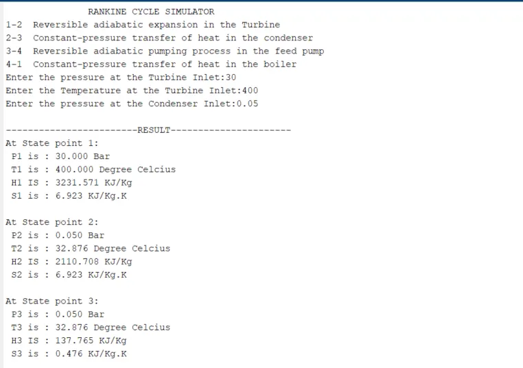
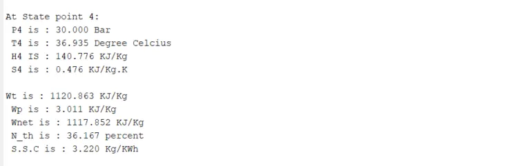
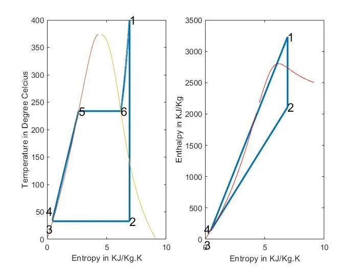
ERRORS :
- The process (1-2) is not isentropic
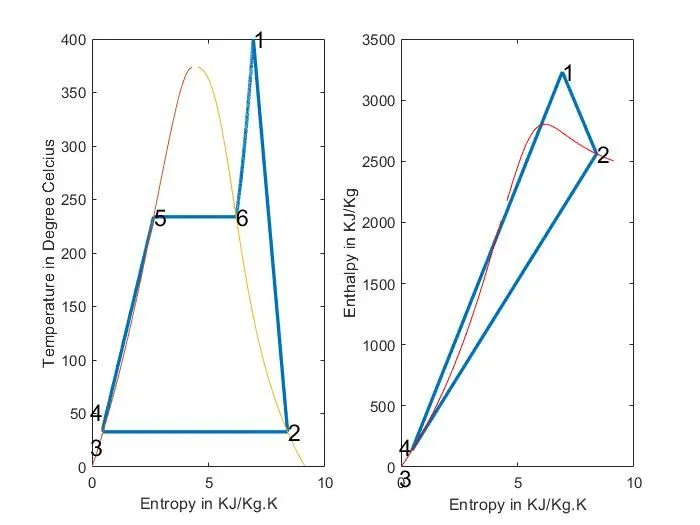
This error occurs when we considered s2 = sg2 that means we assumed x2 = 1. To correct that error, the correct equation to be used is s2 = sf2 + x2*(sg2 - sf2). It implies that x2 = (s2-sf2)/(sg2-sf2)
REFERENCES:
- Thermal Engineering book by Er. R.K. Rajput, Tenth Edition
- Thermodynamics Demystified book by Merle C. Potter, Ph.D.
- https://www.intechopen.com/books/organic-rankine-cycle-technology-for-heat-recovery/the-development-and-application-of-organic-rankine-cycle-for-vehicle-waste-heat-recovery
- https://www.instructables.com/Simple-Rankine-Cycle-Thermodynamics/
- http://www.thermix.net/2012/06/blog-post.html