Week 3 - Adiabatic Flame Temperature calculation
Aim: To calculate adiabatic flame temperature variation with respect to:
- Equivalence ratio in constant volume-chamber
- Heat loss in constant pressure-chamber
- Alkane, Alkene and Alkyne
- Number of carbon atom chains
Introduction
The temperature of the products for a combustion taking place under adiabatic conditions is referred to as the adiabatic flame temperature. Usually, it is the highest temperature that can be achieved. In fact, an exothermic chemical reaction releases heat to its products during combustion, thereby raising their temperature. There is no possibility for dissipation of the heat to the surrounding and the process will be adiabatic as there is no heat loss to the surrounding. As a result, the temperature of the products suddenly increases and it produces a flame. This will heat up the product gases in flame region and the temperature rise will be maximum. This highest temperature is known as the adiabatic flame temperature. The temperature rise depends on the amount of excess air used or the air-fuel ratio. The flame temperature has the highest value for using pure oxygen gas and it decreases by using air. So, the exact stoichiometric air is to be supplied for better result. With too large amount of excess air the flame temperature will be reduced. When the heat loss to the environment or diluted by the inert gases and there is an incomplete combustion. So, the temperature of the products will be less. The flame temperature is determined from the energy balance of the reaction at equilibrium. There are two type of adiabatic flame temperature: constant pressure adiabatic flame temperature and constant volume adiabatic flame temperature. The main objective of this work is to learn and understand how the adiabatic flame temperature is influenced by different factors and get learn the basic concepts of Cantera as well as Python programming.
Theory:
As stated earlier, depending on how the process is completed, adiabatic flame temperature can be of constant volume or constant pressure type as shown following:
According to the first law of thermodynamics for a closed reacting system, we have:
`Q-W=U_P-U_R`
Where Q and W are the heat and work transferred during the process respectively and Up and Ur are the internal energy of the products and reactants respectively.
- Constant volume combustion
In the constant volume adiabatic flame temperature, the volume of the system is held constant as the name suggested; hence there is no work occurring. We then have:
`W= ∫_R^PpdV=0` and there is no heat transfer because the process is defined to be adiabatic: . Consequently, the internal energy of the products is equal to the internal energy of the reactants: . Since this is a closed system, the mass of the products and reactants is constant and the first law can be written on a mass basis as follows: `U_P=U_R→m_P u_P=m_R u_R→u_P=u_R`
- Constant pressure combustion
In the constant pressure adiabatic flame temperature case, the pressure of the system is held constant which results in the following equation for the work:
`W= ∫_R^PpdV=p(V_P-V_R )`
Moreover, there is no heat transfer occurring because the process is defined to be adiabatic Q = 0. From the first law, we find that
`-p(V_P-V_R )=U_P-U_R→U_P+pV_P=U_R+ pV_R`
Recalling the definition of the enthalpy we recover. Because this is a closed system the mass of the products and reactants is constant and the first law can be written on a mass basis as follows:
`H_P=H_R→m_P h_P= m_R h_R→h_P=h_R`
As it can be seen, the adiabatic flame temperature of the constant pressure process is lower than that of the constant volume process. This is because some of the energy released during the combustion goes into changing the volume of the control system. One analogy commonly made between the two processes is through combustion in an internal combustion engine. For the constant volume adiabatic process, combustion is thought to occur instantaneously when the piston reaches the top of its apex (Otto cycle or constant volume cycle). For the constant pressure adiabatic process, while combustion is occurring the piston is moving in order to keep the pressure constant (Diesel cycle or constant pressure cycle)
- Concepts of Air-Fuel mixture
Stoichiometric combustion: The air-fuel ratio for complete combustion is called stoichiometric air-fuel ratio.
Equivalence Ratio: The air-fuel equivalence ratio (ф) of a system is defined as the ratio of the fuel to oxidizer ratio to the stoichiometric fuel to oxidizer ratio. It measures how a mixture is deviating from an ideal stoichiometric reaction. When ф = 1, the combustion reaction is termed as stoichiometric.
`ф= ((m_fuel)/(m_air) )_(actual mixture)/((m_fuel)/(m_air ))_(stoichiometric mixture)`
Lean mixture: When the amount of air is more than the amount of fuel for a complete reaction, the mixture is termed as lean mixture. It is characterized by ф < 1.
Rich Mixture: When the amount of air is less than the amount of fuel for complete combustion, the mixture is termed as rich mixture. It is characterized by ф > 1.
CASE 1: EFFECT OF EQUIVALENCE RATIO ON AFT FOR CONSTANT VOLUME COMBUSTION PROCESS OF METHANE
For a constant volume process, internal energy is equated for reactants and products to get AFT, U_r - U_p = 0. Using Newton Raphson method, the final temperature is obtained as shown:
(Hproducts - n_products*R*T) – (Hreactants - n_products*R*Tstd )
`H=((a1 + a2*T/2 + a3*pow(T,2)/3 + a4*pow(T,3)/4 + a5*pow(T,4)/5 + a6/T))*R*T`
The equivalence ratio is varied from 0.1 to 2.
"""
In this program we are going to calculate the AFT of Methane at different equivalence ratios

CH4 + 2(O2 + 3.76N2) = CO2 + 2H2O + 7.52N2
Lean Mixture
CH4 + (2/phi)(O2 + 3.76N2) = CO2 + 2H2O + (7.52/phi)N2 + (2/phi-2)O2
Rich mixture
CH4 + (2/phi)(O2 + 3.76N2) = (4/phi-3)CO2 + 2H2O + (7.52/phi)N2 + (4-4/phi)CO

Program by - MAckly

"""


import matplotlib.pyplot as plt
import math
import numpy as np
import cantera as ct
R = 8.314

def h(T, co_effs):
	"""

	Function to evaluate enthalpy

	"""
	R = 8.314 # J/mol-K
	a1 = co_effs[0]
	a2 = co_effs[1]
	a3 = co_effs[2]
	a4 = co_effs[3]
	a5 = co_effs[4]
	a6 = co_effs[5]


	return ((a1 + a2*T/2 + a3*pow(T,2)/3 + a4*pow(T,3)/4 + a5*pow(T,4)/5 + a6/T))*R*T


#Low temperature coefficients
ch4_coeffs_l = [5.14987613E+00,-1.36709788E-02,4.91800599E-05,-4.84743026E-08,1.66693956E-11,-1.02466476E+04,-4.64130376E+00]

o2_coeffs_l = [3.78245636E+00,-2.99673416E-03,9.84730201E-06,-9.68129509E-09,3.24372837E-12,-1.06394356E+03,3.65767573E+00]

n2_coeffs_l = [0.03298677E+02,0.14082404E-02,-0.03963222E-04,0.05641515E-07,-0.02444854E-10,-0.10208999E+04,0.03950372E+02]

#High temperature coefficients
n2_coeffs_h = [0.02926640E+02,0.14879768E-02,-0.05684760E-05,0.10097038E-09,-0.06753351E-13,-0.09227977E+04,0.05980528E+02]

co2_coeffs_h = [3.85746029E+00,4.41437026E-03,-2.21481404E-06,5.23490188E-10,-4.72084164E-14,-4.87591660E+04,2.27163806E+00]

h2o_coeffs_h = [3.03399249E+00,2.17691804E-03,-1.64072518E-07,-9.70419870E-11,1.68200992E-14,-3.00042971E+04,4.96677010E+00]

o2_coeffs_h = [3.28253784E+00, 1.48308754E-03,-7.57966669E-07,2.09470555E-10,-2.16717794E-14,-1.08845772E+03,5.45323129E+00]

co_coeffs_h = [2.71518561E+00,2.06252743E-03,-9.98825771E-07,2.30053008E-10,-2.03647716E-14,-1.41518724E+04,7.81868772E+00]


def f(T,phi):
	"""
	Function that represents the Root finding problem
	"""

	h_co2_p = h(T,co2_coeffs_h)
	h_n2_p = h(T,n2_coeffs_h)
	h_h2o_p = h(T,h2o_coeffs_h)
	h_o2_p = h(T,o2_coeffs_h)
	h_co_p = h(T,co_coeffs_h)


#Lean mixture enthalpy calculation
	if phi < 1:
		H_products = h_co2_p + 2*h_h2o_p + (7.52/phi)*h_n2_p + (2/phi-2)*h_o2_p

		n_products = 1 + 2 + (7.52/phi) + (2/phi-2)


	if phi == 1:
		H_products = h_co2_p + 2*h_h2o_p + 7.52*h_n2_p
		n_products = 1 + 2 + 7.52

	if phi > 1:
		H_products = (4/phi - 3)*h_co2_p + 2*h_h2o_p + (7.52/phi)*h_n2_p + (4 - 4/phi)*h_co_p
		n_products = (4/phi - 3) + 2 + 7.52/phi + (4 - 4/phi)


	Tstd = 298.15
	h_ch4_r = h(Tstd,ch4_coeffs_l)
	h_o2_r = h(Tstd,o2_coeffs_l)
	h_n2_r = h(Tstd,n2_coeffs_l)

	H_reactants = h_ch4_r + (2/phi)*(h_o2_r + 3.76*h_n2_r)
	n_reactants = 1 + 2/phi + 7.52/phi


	return (H_reactants - n_reactants*R*Tstd)-(H_products - n_products*R*T)


def fprime(T,phi):
	return (f(T+1e-6,phi)-f(T,phi))/1e-6

T_guess = 1500

tol = 1e-6
#ct = 0
alpha = 0.2
PHI = np.arange(0.1,2,0.03)
T_ad = []

for phi in PHI:

	while (abs(f(T_guess,phi)) > tol):
		T_guess = T_guess - alpha*((f(T_guess,phi)/fprime(T_guess,phi)))

	T_ad.append(T_guess)

plt.plot(PHI,T_ad,'*-',color = 'red',label = "using newton raphson")
plt.grid('on')


"""
Using Cantera
"""
gas = ct.Solution('gri30.xml')
T_aft_ct = []

for phi in PHI:

	#Computing the mole fraction of each reactant

	n_total = 1 + (2/phi) + (7.52/phi)
	n_ch4 = 1/(n_total)
	n_o2 = 2/(phi*n_total)
	n_n2 = 7.52/(phi*n_total)

	#Defining of gas mixture

	#gas.TPX = 298.15,101325, {'CH4':n_ch4, 'O2':n_o2, 'N2':n_n2}
	gas.TPX = 298.15,101325, {'CH4':1, 'O2':2/phi, 'N2':7.52/phi}

	#Computation of equilibrium conditions

	gas.equilibrate('UV', 'auto')
	T_aft_ct.append(gas.T)
#print(T_aft_ct)


#Plotting the results
plt.plot(PHI,T_aft_ct,'-o',color='blue',label="Using Cantera")
plt.xlabel('Equivalence Ratio')
plt.ylabel('Adiabatic Flame Temperature')
plt.title('Effect of Equivalence Ratio on AFT of Methane')
plt.legend()
plt.show()
RESULTS:
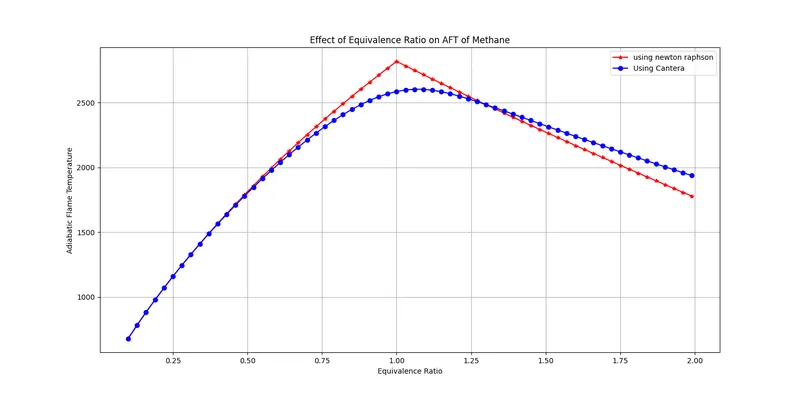
As it can be seen on the graphs, the AFT at stoichiometric condition (phi = 1) is higher. As we go beyond phi = 1, the AFT starts decreasing drastically. This is because at stoichiometric conditions, the whole fuel is burnt and consequently, more energy is produced. This variation is quite same for both graphs. Now, comparing these two graphs, we can see that the graph obtained from Newton Raphson Method is above the one obtained from Cantera. This is explained by the fact that Cantera uses all products of the combustion so more energy is consumed to produce these products hence the AFT is lower in that case which is the correct or accurate result.
CASE 2: ADIABATIC FLAME TEMPERATURE Vs HEAT LOSS
For a constant pressure combustion process, enthalpy is equated for reactants and products to obtain the AFT as shown below:
H_r -H_p + Heat_Loss = 0
The maximum possible heat loss is the lower heat value (LHV) which is given by Heat_loss_Factor*(LHV). Enthalpy is computed using the same formula as previously. The heat loss is varied from 0 to 1.
"""
In this program we are going to compute the variation of AFT with the heat loss

CH4 + 2(O2 + 3.76N2) = CO2 + 2H2O + 7.52N2


Program by - MAckly

"""


import matplotlib.pyplot as plt
import math
import numpy as np

R = 8.314
Tstd = 298.15

def h(T, co_effs):
	"""

	This Function has to evaluate enthalpy of different species

	"""
	R = 8.314 # J/mol-K
	a1 = co_effs[0]
	a2 = co_effs[1]
	a3 = co_effs[2]
	a4 = co_effs[3]
	a5 = co_effs[4]
	a6 = co_effs[5]


	return ((a1 + a2*T/2 + a3*pow(T,2)/3 + a4*pow(T,3)/4 + a5*pow(T,4)/5 + a6/T))*R*T


#Low temperature coefficients
ch4_coeffs_l = [5.14987613E+00,-1.36709788E-02,4.91800599E-05,-4.84743026E-08,1.66693956E-11,-1.02466476E+04,-4.64130376E+00]

o2_coeffs_l = [3.78245636E+00,-2.99673416E-03,9.84730201E-06,-9.68129509E-09,3.24372837E-12,-1.06394356E+03,3.65767573E+00]

n2_coeffs_l = [0.03298677E+02,0.14082404E-02,-0.03963222E-04,0.05641515E-07,-0.02444854E-10,-0.10208999E+04,0.03950372E+02]

#High temperature coefficients
n2_coeffs_h = [0.02926640E+02,0.14879768E-02,-0.05684760E-05,0.10097038E-09,-0.06753351E-13,-0.09227977E+04,0.05980528E+02]

co2_coeffs_h = [3.85746029E+00,4.41437026E-03,-2.21481404E-06,5.23490188E-10,-4.72084164E-14,-4.87591660E+04,2.27163806E+00]

h2o_coeffs_h = [3.03399249E+00,2.17691804E-03,-1.64072518E-07,-9.70419870E-11,1.68200992E-14,-3.00042971E+04,4.96677010E+00]


#Computing The Low Heating Value

LHV = h(Tstd,ch4_coeffs_l) + 2*h(Tstd,o2_coeffs_l) - h(Tstd,co2_coeffs_h) - 2*h(Tstd,h2o_coeffs_h)

def f(T,Heat_loss):

	"""
	Function that represents the Root finding problem
	"""

	h_co2_p = h(T,co2_coeffs_h)
	h_n2_p = h(T,n2_coeffs_h)
	h_h2o_p = h(T,h2o_coeffs_h)

	H_products = h_co2_p + 2*h_h2o_p + 7.52*h_n2_p


	#Tstd = 298.15
	h_ch4_r = h(Tstd,ch4_coeffs_l)
	h_o2_r = h(Tstd,o2_coeffs_l)
	h_n2_r = h(Tstd,n2_coeffs_l)

	H_reactants = h_ch4_r + 2*(h_o2_r + 3.76*h_n2_r)
	#n_reactants = 1 + 2/phi + 7.52/phi


	return (H_products - H_reactants + (Heat_loss*LHV))


def fprime(T,Heat_loss):

	return (f(T+1e-6,Heat_loss)-f(T,Heat_loss))/1e-6


T_guess = 1500
tol = 1e-6
alpha = 0.2
H_L = np.arange(0,1,0.05)
T_ad = []

for Heat_loss in H_L:

	while (abs(f(T_guess,Heat_loss)) > tol):
		T_guess = T_guess - alpha*((f(T_guess,Heat_loss)/fprime(T_guess,Heat_loss)))

	T_ad.append(T_guess)


#Plotting the results

plt.plot(H_L,T_ad,'*-',color = 'red',label = "using newton raphson")
plt.grid('on')
plt.xlabel('Heat Loss Factor')
plt.ylabel('Adiabatic Flame Temperature')
plt.title('Effect of Heat Loss on AFT of Methane')
plt.legend()
plt.show()
RESULTS
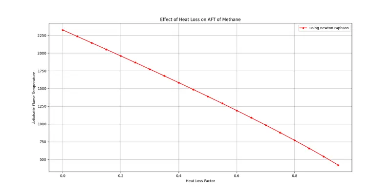
We can see that the AFT decreases with increase in heat loss. This is because less energy is contained in combustion chamber hence the decrease in final temperature.
CASE 3: ADIABATIC FLAME TEMPERATURE VARIRATION WITH RESPECT TO ALKANE, ALKENE & ALKYNE
For this case, the same procedure as previously is followed for 2 carbon atoms hydrocarbons which are Ethane, Ethene and Ethyne.
"""
In this program we are going to compute the variation of AFT with respect to Alkane, Alkene
and Alkyne for number of carbon atom = 2 (C=2)

The general formula used is as follows:
CxHy + [x+(y/4)](O2 + 3.76N2) ==>  xCO2 + (y/2)H2O + 3.76[x+(y/4)]N2

For ETHANE: C2H6 + 3.5(O2 + 3.76N2) ==>  2CO2 + 3H2O + 13.16N2

For ETHENE: C2H4 + 3(O2 + 3.76N2) ==>  2CO2 + 2H2O + 11.28N2

For ETHYNE: C2H2 + 2.5(O2 + 3.76N2) ==>  2CO2 + H2O + 9.4N2

Program by - Abouzi

"""


import matplotlib.pyplot as plt
import math
import numpy as np

R = 8.314
Tstd = 298.15


def h(T, co_effs):
	"""

	This Function has to evaluate enthalpy of different species

	"""
	R = 8.314 # J/mol-K
	a1 = co_effs[0]
	a2 = co_effs[1]
	a3 = co_effs[2]
	a4 = co_effs[3]
	a5 = co_effs[4]
	a6 = co_effs[5]


	return ((a1 + a2*T/2 + a3*pow(T,2)/3 + a4*pow(T,3)/4 + a5*pow(T,4)/5 + a6/T))*R*T


#Low temperature coefficients

c2h6_coeffs_l = [4.29142492E+00,-5.50154270E-03,5.99438288E-05,-7.08466285E-08,2.68685771E-11,-1.15222055E+04,2.66682316E+00]

c2h4_coeffs_l= [3.95920148E+00,-7.57052247E-03,5.70990292E-05,-6.91588753E-08,2.69884373E-11,5.08977593E+03,4.09733096E+00]

c2h2_coeffs_l = [8.08681094E-01,2.33615629E-02,-3.55171815E-05,2.80152437E-08,-8.50072974E-12,2.64289807E+04,1.39397051E+01]

o2_coeffs_l = [3.78245636E+00,-2.99673416E-03,9.84730201E-06,-9.68129509E-09,3.24372837E-12,-1.06394356E+03,3.65767573E+00]

n2_coeffs_l = [0.03298677E+02,0.14082404E-02,-0.03963222E-04,0.05641515E-07,-0.02444854E-10,-0.10208999E+04,0.03950372E+02]


#High temperature coefficients

n2_coeffs_h = [0.02926640E+02,0.14879768E-02,-0.05684760E-05,0.10097038E-09,-0.06753351E-13,-0.09227977E+04,0.05980528E+02]

co2_coeffs_h = [3.85746029E+00,4.41437026E-03,-2.21481404E-06,5.23490188E-10,-4.72084164E-14,-4.87591660E+04,2.27163806E+00]

h2o_coeffs_h = [3.03399249E+00,2.17691804E-03,-1.64072518E-07,-9.70419870E-11,1.68200992E-14,-3.00042971E+04,4.96677010E+00]

o2_coeffs_h = [3.28253784E+00, 1.48308754E-03,-7.57966669E-07,2.09470555E-10,-2.16717794E-14,-1.08845772E+03,5.45323129E+00]

co_coeffs_h = [2.71518561E+00,2.06252743E-03,-9.98825771E-07,2.30053008E-10,-2.03647716E-14,-1.41518724E+04,7.81868772E+00]


def f(T,typee):

	"""
	Function that represents the Root finding problem
	"""

	h_co2_p = h(T,co2_coeffs_h)
	h_n2_p = h(T,n2_coeffs_h)
	h_h2o_p = h(T,h2o_coeffs_h)


	h_c2h6_r = h(Tstd,c2h6_coeffs_l)
	h_c2h4_r = h(Tstd,c2h4_coeffs_l)
	h_c2h2_r = h(Tstd,c2h2_coeffs_l)
	h_o2_r = h(Tstd,o2_coeffs_l)
	h_n2_r = h(Tstd,n2_coeffs_l)

	if typee == 1:

		x = 2
		y = 6

		H_Fuel = h_c2h6_r

	elif typee == 2:

		x = 2
		y = 4

		H_Fuel = h_c2h4_r

	elif typee == 3:

		x = 2
		y = 2

		H_Fuel = h_c2h2_r

	H_products = x*h_co2_p + (y/2)*h_h2o_p + 3.76*(x + y/4)*h_n2_p

	H_reactants = H_Fuel + (x + y/4)*h_o2_r + 3.76*(x + y/4)*h_n2_r

	return (H_products - H_reactants)


def fprime(T,typee):

	return (f(T+1e-6,typee)-f(T,typee))/1e-6


T_guess = 1500
tol = 1e-6
alpha = 0.2
typee = [1,2,3]
T_ad = []

for i in typee:

	while (abs(f(T_guess,i)) > tol):

		T_guess = T_guess - alpha*((f(T_guess,i)/fprime(T_guess,i)))

	T_ad.append(T_guess)


#Plotting the results

plt.bar(['Ethane($C_2H_6$)','Ethene($C_2H_4$)','Ethyne($C_2H_2$)'],T_ad)
#plt.grid('on')
#plt.xlabel('Heat Loss Factor')
plt.ylabel('Adiabatic Flame Temperature')
plt.title('Effect of Heat Loss on AFT of Methane')
plt.legend()
plt.show()
RESULTS
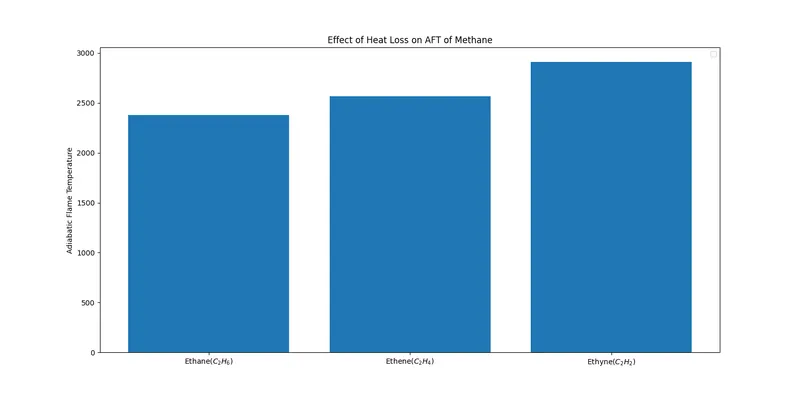
As it can be seen, the lowest AFT is obtained in case of Ethane which is alkane and the highest AFT is obtained in case of Ethyne which is Alkyne. This is explained by the fact that Alkanes contain one Carbon-Carbon bond whereas in case of Alkynes, they contain three Carbon-Carbon bonds which require more energy to break hence the highest AFT.
CASE 4: ADIABATIC FLAME TEMPERATURE VARIATION WITH RESPECT TO NUMBER OF CARBON ATOM CHAINS
In this case, the number of carbon atoms is varied from 1 to 3. The corresponding hydrocarbons are Methane, Ethane and Propane.
"""
In this program we are going to compute the variation of AFT of Alkane with number
of carbon atoms varying from 1 to 3

METHANE: CH4 + 2(O2 + 3.76N2) = CO2 + 2H2O + 7.52N2

ETHANE: C2H6 + 3.5(O2 + 3.76N2) = 2CO2 + 3H2O + 13.16N2

PROPANE: C3H4 + 2(O2 + 3.76N2) = CO2 + 2H2O + 7.52N2


Program by - Abouzi

"""


import matplotlib.pyplot as plt
import math
import numpy as np


R = 8.314
Tstd = 298.15


def h(T, co_effs):
	"""

	Function to evaluate enthalpy

	"""
	R = 8.314 # J/mol-K
	a1 = co_effs[0]
	a2 = co_effs[1]
	a3 = co_effs[2]
	a4 = co_effs[3]
	a5 = co_effs[4]
	a6 = co_effs[5]


	return ((a1 + a2*T/2 + a3*pow(T,2)/3 + a4*pow(T,3)/4 + a5*pow(T,4)/5 + a6/T))*R*T


#Low temperature coefficients

ch4_coeffs_l = [5.14987613E+00,-1.36709788E-02,4.91800599E-05,-4.84743026E-08,1.66693956E-11,-1.02466476E+04,-4.64130376E+00]

c2h6_coeffs_l = [4.29142492E+00,-5.50154270E-03,5.99438288E-05,-7.08466285E-08,2.68685771E-11,-1.15222055E+04,2.66682316E+00]

c3h8_coeffs_l = [0.93355381E+00,0.26424579E-01,0.61059727E-05,-0.21977499E-07,0.95149253E-11,-0.13958520E+05,0.19201691E+02]

o2_coeffs_l = [3.78245636E+00,-2.99673416E-03,9.84730201E-06,-9.68129509E-09,3.24372837E-12,-1.06394356E+03,3.65767573E+00]

n2_coeffs_l = [0.03298677E+02,0.14082404E-02,-0.03963222E-04,0.05641515E-07,-0.02444854E-10,-0.10208999E+04,0.03950372E+02]


#High temperature coefficients

n2_coeffs_h = [0.02926640E+02,0.14879768E-02,-0.05684760E-05,0.10097038E-09,-0.06753351E-13,-0.09227977E+04,0.05980528E+02]

co2_coeffs_h = [3.85746029E+00,4.41437026E-03,-2.21481404E-06,5.23490188E-10,-4.72084164E-14,-4.87591660E+04,2.27163806E+00]

h2o_coeffs_h = [3.03399249E+00,2.17691804E-03,-1.64072518E-07,-9.70419870E-11,1.68200992E-14,-3.00042971E+04,4.96677010E+00]


def f(T,typee):
	"""
	Function that represents the Root finding problem
	"""

	h_co2_p = h(T,co2_coeffs_h)
	h_n2_p = h(T,n2_coeffs_h)
	h_h2o_p = h(T,h2o_coeffs_h)


	h_ch4_r = h(Tstd,ch4_coeffs_l)
	h_c2h6_r = h(Tstd,c2h6_coeffs_l)
	h_c3h8_r = h(Tstd,c3h8_coeffs_l)
	h_o2_r = h(Tstd,o2_coeffs_l)
	h_n2_r = h(Tstd,n2_coeffs_l)

	if typee == 1:

		x = 1

		y = 4

		H_fuel = h_ch4_r

	elif typee == 2:

		x = 2

		y = 6

		H_fuel = h_c2h6_r

	elif typee == 3:

		x = 3

		y = 8

		H_fuel = h_c3h8_r


	H_products = x*h_co2_p + (y/2)*h_h2o_p + 3.76*(x + y/4)*h_n2_p

	H_reactants = H_fuel + (x + y/4)*h_o2_r + 3.76*(x + y/4)*h_n2_r

	return (H_products - H_reactants)


def fprime(T,typee):
	return (f(T+1e-6,typee)-f(T,typee))/1e-6


T_guess = 1500
tol = 1e-6
alpha = 0.2
typee = [1,2,3]
T_ad = []


for i in range(0,len(typee)):


	while (abs(f(T_guess,typee[i])) > tol):

		T_guess = T_guess - alpha*((f(T_guess,typee[i])/fprime(T_guess,typee[i])))

	T_ad.append(T_guess)

plt.bar(['Methane($CH_4$)','Ethane($C_2H_6$)','Propane($C_3H_8$)'],T_ad)

plt.ylabel('Adiabatic Flame Temperature')
plt.title('Effect of carbon atom number on AFT of Alkane')
plt.legend()
plt.show()
RESULTS
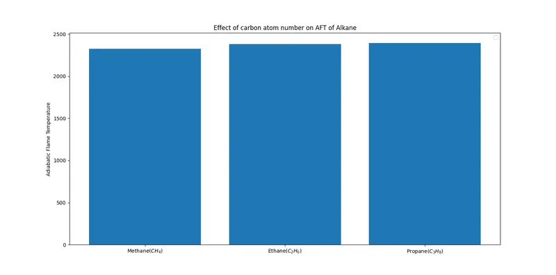
From the above bar chart, we can see that the AFT increases with increase in the number of Carbon atoms. Thus, the highest AFT is obtained for Propane and the lowest AFT from Methane. We can then say that, the adiabatic flame temperature increases with increase in number of carbon atoms for Alkane hydrocarbons group.
CONCLUSION
Finally, the adiabatic flame temperature is computed with its variation with respect to Equivalence ratio in constant volume-chamber, Heat loss in constant pressure-chamber, Alkane, Alkene and Alkyne, Number of carbon atom chains for Alkane hydrocarbons group. Different observations were done and conclusions are stated for each case.
References