Deriving 4th order approximation of a 2nd order derivative using Taylor Table method

AIM: To derive the 4^th order approximations of the second order derivative using central difference method, skewed right-sided difference method and skewed left-sided difference.

OBJESCTIVES:

• Learn the concept of Taylor table and its importance,
• To determine the difference between central and one-sided schemes by comparing them,
• To understand the importance of skewed.

EQUATIONS AND TERMS USED:

• `f(x)=f^' (x_0 )(x-x_0 )+(f'' (x_0 ))/(2!) (x-x_0)^2+(f''' (x_0 ))/(3!) (x-x_0)^3+(f'''' (x_0 ))/(4!) (x-x_0)^4+⋯=∑_(n=0)^∞(f^((n) ) (x_0 ))/(n!) (x-x_0 )^n.`

This is Taylor series of the function f(x).

• The order of accuracy(P): It is the power of dx with which the truncation error tends to zero. Here that order is taken as 4.
• The order of derivative(Q): As known, Differential equations are classified on the basis of the order. So, the order of a differential is the order of its highest derivative.
• Number of nodes(N): Nodes are specified data points at which the approximation method matches a given function f. So, the number of nodes is the total number of data points needed to perform an approximation.
• Stencil: It is a geometric arrangement of a nodal group that relate to the point of interest by using a numerical approximation routine.

• Central difference (CD)

For fourth order approximation, N =P+Q-1= 4+2-1. Hence a five points stencil is used with nodes indices as follows: i-2, i-1, i, i+1 and i+2.

Thus, the second order derivative of 4^th approximation for central difference scheme (CDS) is written as:

`(∂^2 f)/(∂x)^2 =af(i-2)+bf(i-1)+cf(i)+df(i+1)+ef(i+2)`

After expanding each term using Taylor series formula, following Taylor table is obtained:

Stencil	f(i)	dxf’(i)	`(dx)^2 f'' (i)`	`(dx)^3 f''' (i)`	`(dx)^4 f'''' (i)`
af(i-2)	a	-2a	2a	-8a/6	16a/24
bf(i-1)	b	-b	b/2	-b/6	b/24
cf(i)	c	0	0	0	0
df(i+1)	d	d	d/2	d/6	d/24
ef(i+2)	e	2e	2e	8e/6	16e/24
	0	0	1	0	0

• Skewed right-sided difference (SRSD)

For fourth order approximation, N = P+Q=4+2.

Thus, a six points stencil is used with nodes indices as follows: i, i+1, i+2, i+3, i+4, i+5.

The second order derivative of 4^th approximation for SRSD is written as:

`(∂^2 f)/(∂x)^2 =af(i)+bf(i+1)+cf(i+2)+df(i+3)+ef(i+4)+gf(i+5)`

After expanding each term using Taylor series formula, following Taylor table is obtained:

Stencil	f(i)	dxf’(i)	`(dx)^2 f'' (i)`	`(dx)^3 f''' (i)`	`(dx)^4 f'''' (i)`	`(dx)^5 f''''' (i)`
af(i)	a	0	0	0	0	0
bf(i+1)	b	b	b/2	b/6	b/24	b/120
cf(i+2)	c	2c	2c	8c/6	16c/24	32c/120
df(i+3)	d	3d	9d/2	27d/6	81d/24	243d/120
ef(i+4)	e	4e	16e/2	64e/6	256e/24	1024e/120
gf(i+5)	g	5g	25g/2	125g/6	625g/24	3125g/120
	0	0	1	0	0	0

• Skewed left-sided difference (SLSD)

Here, for the fourth order approximation, N=P+Q=4+2.

Hence a six-points stencil used with node indices as follows: i-5, i-4, i-3, i-2, i-1, i.

The second order derivative of 4^th approximation for SLSD is written as:

`(∂^2 f)/(∂x)^2 =af(i-5)+bf(i-4)+cf(i-3)+df(i-2)+ef(i-1)+gf(i)`

After expanding each term using Taylor series formula, following Taylor table is obtained:

Stencil	f(i)	dxf’(i)	`(dx)^2 f'' (i)`	`(dx)^3 f''' (i)`	`(dx)^4 f'''' (i)`	`(dx)^5 f''''' (i)`
af(i-5)	a	-5a	25a/2	-125a/6	625a/24	-3125a/120
bf(i-4)	b	-4b	16b/2	-64b/6	256b/24	-1024b/120
cf(i-3)	c	-3c	9c/2	-27c/6	81c/24	-243c/120
df(i-2)	d	-2d	2d	-8d/6	16d/24	-32d/120
ef(i-1)	e	-e	e/2	-e/6	e/24	-e/120
gf(i)	g	0	0	0	0	0
	0	0	1	0	0	0

MATLAB Program to evaluate the second order derivative

• Program function 1: “central_diff(x,dx)”

%This function calculates the error for central difference method 
function out1 = central_diff(x,dx)
%Analytical function is f(x) = exp(x)*cos(x)
%Calculation of the approximation coefficients using matrix inversion
%method
a = [1 1 1 1 1;-2 -1 0 1 2;2 1/2 0 1/2 2;-8/6 -1/6 0 1/6 8/6;16/24 1/24 0 1/24 16/24];
b = [0;0;1;0;0];
%central_diff_coeff = inv(a)*b;
central_diff_coeff = ab;
%Analytical_derivative is f''(x) = -2*sin(x)*exp(x)
Analytical_derivative = -2*sin(x)*exp(x);

%Calculation of the error
central_differencing = (central_diff_coeff(1)*exp(x-2*dx)*cos(x-2*dx)+central_diff_coeff(2)*exp(x-dx)*cos(x-dx)+central_diff_coeff(3)*exp(x)*cos(x)+central_diff_coeff(4)*exp(x+dx)*cos(x+dx)+central_diff_coeff(5)*exp(x+2*dx)*cos(x+2*dx))/((dx)^2);

out1 = abs(central_differencing-Analytical_derivative);

end

The coefficients values for

`(∂^2 f)/(∂x)^2 =af(i-2)+bf(i-1)+cf(i)+df(i+1)+ef(i+2)`

are:

a= 0.083333333333334

b=1.333333333333334

c=2.500000000000001

d=1.333333333333334

e=0.083333333333334

Program function 2: “skewed_right_sided_diff(x,dx)”

%This program calculates the error for the skewed right-sided difference
function out2 = skewed_right_sided_diff(x,dx)
%Analytical function is f(x) = exp(x)*cos(x)
%Calculation of the approximation coefficients using matrix inversion
%method
R = [1 1 1 1 1 1;0 1 2 3 4 5;0 1/2 2 9/2 16/2 25/2;0 1/6 8/6 27/6 64/6 125/6;0 1/24 16/24 81/24 256/24 625/24;0 1/120 32/120 243/120 1024/120 3125/120];
S = [0;0;1;0;0;0];
%right_side_diff_coeff = inv(R)*S;
right_sided_diff_coeff = RS;
%Analytical_derivative is f''(x) = -2*sin(x)*exp(x)
Analytical_derivative = -2*sin(x)*exp(x);

%Calculation of the error
Right_sided_differencing = (right_sided_diff_coeff(1)*exp(x)*cos(x)+right_sided_diff_coeff(2)*exp(x+dx)*cos(x+dx)+right_sided_diff_coeff(3)*exp(x+2*dx)*cos(x+2*dx)+right_sided_diff_coeff(4)*exp(x+3*dx)*cos(x+3*dx)+right_sided_diff_coeff(5)*exp(x+4*dx)*cos(x+4*dx)+right_sided_diff_coeff(6)*exp(x+5*dx)*cos(x+5*dx))/((dx)^2);

out2 = abs(Right_sided_differencing-Analytical_derivative);
end

The coefficients values for

`(∂^2 f)/(∂x)^2 =af(i)+bf(i+1)+cf(i+2)+df(i+3)+ef(i+4)+gf(i+5)`

are:

a= 3.750000000000021

b=12.833333333333435

c=17.833333333333520

d=13.000000000000170

e=5.083333333333411

g=0.833333333333348

Program function 3: “skewed_left_sided_diff(x,dx)”

%This program calculates the error for the skewedn left-sided difference

function out3 = skewed_left_sided_diff(x,dx)
%Analytical function is f(x) = exp(x)*cos(x)
%Calculation of the approximation coefficients using matrix inversion
%method
T = [1 1 1 1 1 1;-5 -4 -3 -2 -1 0;25/2 16/2 9/2 2 1/2 0;-125/6 -64/6 -27/6 -8/6 -1/6 0;625/24 256/24 81/24 16/24 1/24 0;-3125/120 -1024/120 -243/120 -32/120 -1/120 0];
V = [0;0;1;0;0;0];
%left_side_diff_coeff = inv(T)*V;
left_sided_diff_coeff = TV;
%Analytical_derivative is f''(x) = -2*sin(x)*exp(x)
Analytical_derivative = -2*sin(x)*exp(x);

%Calculation of the error
Right_side_differencing = (left_sided_diff_coeff(1)*exp(x-5*dx)*cos(x-5*dx)+left_sided_diff_coeff(2)*exp(x-4*dx)*cos(x-4*dx)+left_sided_diff_coeff(3)*exp(x-3*dx)*cos(x-3*dx)+left_sided_diff_coeff(4)*exp(x-2*dx)*cos(x-2*dx)+left_sided_diff_coeff(5)*exp(x-dx)*cos(x-dx)+left_sided_diff_coeff(6)*exp(x)*cos(x))/((dx)^2);

out3 = abs(Right_side_differencing-Analytical_derivative);
end

The coefficients values for

`(∂^2 f)/(∂x)^2 =af(i-5)+bf(i-4)+cf(i-3)+df(i-2)+ef(i-1)+gf(i)`

are:

a= 0.833333333333332

b=5.083333333333323

c=12.999999999999968

d=17.833333333333286

e=12.833333333333304

g=3.749999999999995

MAIN PROGRAM:

clear all
close all
clc

%INPUTS
%Defining the values x and dx
x = pi/3;
dx = linspace(pi/40,pi/4,2000);
%Functios calling for the calculation of different error values under for
%loop
for i =1:length(dx)
  CD_error(i) = central_diff(x,dx(i));
  SR_error(i)= skewed_right_sided_diff(x,dx(i));
  SL_error(i)= skewed_left_sided_diff(x,dx(i));
end
%The commands below are for plottind the different values of errors with
%respect to the range or values of dx.
figure(1)
loglog(dx,CD_error,'g','linewidth',3)
hold on
loglog(dx,SR_error,'r','linewidth',3)
hold on
loglog(dx, SL_error,'b','linewidth',3)
xlabel('dx')
ylabel('error')
legend('Central difference','Skewed right-sided difference','skewed left-sided difference')

EXPLANATION OF CODES LINES:

• These three program functions, take two inputs variables x and dx to return one value as output which is the absolute error between the central difference, skewed right-sided difference, skewed left-sided difference schemes and analytical derivative respectively.
• In each program function, the matrix inversion method is used to calculate the coefficients corresponding to the concerned scheme.
• Then the approximation is determined and the error is computed.
• As for the main program, it is divided into four blocks:

• The first block is about freeing the memory
• The second block is about inputs definition: x and dx; “linspace” command is used to define the range of dx which takes 2000 different values between pi/40 and pi/4.
• The third block is about the calculation of the error’s values for the three schemes. This is done by calling the above three functions within a “for loop”. That “for loop” is to run along the length of dx.
• The fourth and last block deals with the plotting of the error values with respect to dx. Here “loglog” command is used to amplify or enlarge the view.

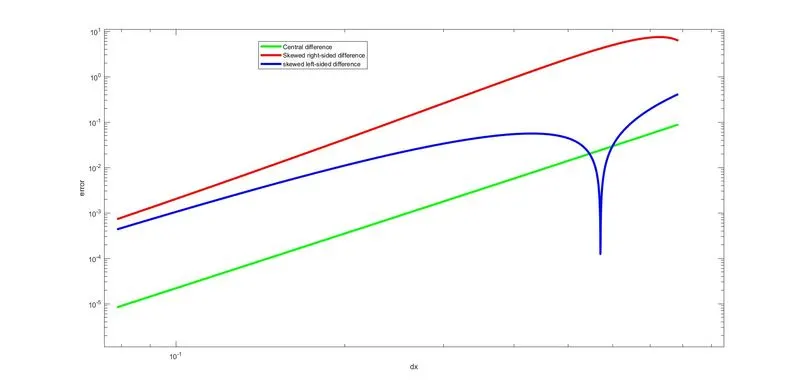
RESULTS/OUTPUT:

EXPLANATION AND ANSWERS TO THE QUESTIONS:

All three schemes are compared to each other as it can be seen on the graph.

By observing the graph, we conclude that

• The skewed right-sided difference gives the maximum error at almost every point of dx.
• The central difference remains consistent throughout the values od dx and it gives the lowest error.
• It is also observed that the skewed left-sided difference is unstable at some point since it gives error below the central difference error.
• Also, when the values of dx are decreased till a certain range, the curves seem to overlap and their ends gets a little bushy. This is due to round off error in MATLAB.

• Why a skewed scheme is useful? What can a skewed scheme do that a CD scheme cannot?

One thing to be noticed is that, in the case of central difference, a central point, surrounded by other two ore more points is considered at which the derivative is computed. But in the case of skewed difference method, the point at which the derivative is to be computed appears to be an end point or a boundary data point. This means, there are other neighbouring data points but only on one side (right side or left side).

So clearly, skewed scheme enables one to compute the numerical derivative at boundary points since CD cannot be used in such cases.

REFERENCES:

• https://en.wikipedia.org/wiki/Stencil_(numerical_analysis)#:~:text=In%20mathematics%2C%20especially%20the%20areas,using%20a%20numerical%20approximation%20routine.