Numerical Analysis of a quasi 1D Subsonic-Supersonic Convergent Divergent Isentropic Nozzle Using MacCormack’s Technique
Abstract
In this project, the simulation of the conditions for an inviscid flow inside a subsonic-supersonic Convergent-Divergent Isentropic Nozzle is done using MacCormack technique. The study is carried out through a quasi-one-dimensional simulation using the finite difference approach in MATLAB. The conservative and non-conservative forms of the governing equations are implemented as well as the Courant number based on time step control. A grid independence test is performed on the solution and the steady-state distribution for the flow-field variables, the time-wise variation along with the variation of Mass flow rate distribution inside the Nozzle are determined and the difference between the two forms of governing equations is investigated by comparing their solutions. The results are plotted with the help of different graphs and it can be concluded after observation that, both conservative and non-conservative forms of governing equations give satisfactory results as per accuracy and convergence consideration.
Introduction
Nozzle is a device designed to control the rate of flow, speed, direction, mass, shape and the pressure of the fluid that exhaust from them. It is of three types namely Convergent nozzle, Divergent nozzle and Convergent-Divergent nozzle that is under study in this work. Thus, a nozzle having a configuration of decreasing area followed by an increasing area is termed as Convergent-Divergent nozzle or CD nozzle. In such nozzle, the hot exhaust leaves the combustion chamber and converges down to the minimum area, or throat of the nozzle. The throat size is chosen to choke the flow and set the mass flow rate through the system. The flow in the throat is sonic which means that the Mach number is equal to one in the throat. Downstream of the throat, the geometry diverges and the flow is isentropically expanded to a supersonic Mach number that depends on the area ratio of the exit to the throat. The expansion of a supersonic flow causes the static pressure and temperature to decrease from the throat to the exit, so the amount of the expansion also determines the exit pressure and temperature. The exit temperature determines the exit speed of sound, which determines the exit velocity. The exit velocity, pressure and mass flow through the nozzle determines the amount of the thrust produced by the nozzle. Throughout this project, the flow is considered to be isentropic. This consideration comes from the assumption that the flow is gradually compressed enabling the flow conditions to return to their original values. Such process is said to be a reversible process which according to second law of thermodynamics, maintains a constant entropy.
The method used in this project is the MacCormack’s technique which is an explicit finite-difference technique of second-order-accurate in both space and time.
Theory and Introduction to the physical problem
We consider the steady, isentropic flow through a convergent-divergent nozzle as sketched in the figure below.
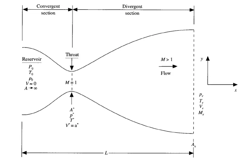
The flow at the inlet to the nozzle comes from a reservoir where the pressure and the temperature are denoted by and respectively.
The cross-sectional area of the reservoir is large (theoretically, A→∞), and hence the velocity is very small (V→0). Thus, and are the stagnation values, or total pressure and total temperature respectively. Then flow expands isentropically to supersonic speeds at the nozzle exit, where the exit pressure temperature, velocity and Mach number are denoted by and , , and respectively. The flow is locally subsonic in the convergent section of the nozzle, sonic flow at the throat means that the local velocity at this location is equal to the local speed od=f sound. Using an asterisk to denote sonic flow values, we have at the throat V = V* = a*. Similarly, the sonic flow values of pressure and temperature are denoted by p* and T* respectively. The area of the sonic throat is denoted by A*. We assume that at a given section, where the cross-sectional area is A, the flow properties are uniform across that section. Hence, although the area of the nozzle changes as a uniform function of distance along the nozzle, x and therefore in reality the flow field is two-dimensional (the flow varies in the two-dimensional xy space), we make the assumption that the flow properties vary only with x; this is tantamount to assuming uniform flow properties across any cross-section.
Governing equations
Since the conservative and non-conservative forms of the governing equations are investigated in this project, the governing continuity, momentum, and energy equation for this quasi-one-dimensional, steady, isentropic flow can be expressed as follows:
- Conservative form
Continuity equation
`(∂(ρA))/(∂t)+(∂(ρAV))/(∂x)=0`
Momentum equation
`(∂(ρAV))/(∂t)+(∂[ρAV^2+1/γ pA])/(∂x)=1/γ p (∂A)/(∂x)`
Energy equation
`(∂[ρ(T/(γ-1)+γ/2 V^2 )A])/(∂t)+(∂[ρ(T/(γ-1)+γ/2 V^2 )VA+pAV])/(∂x)=0`
- Non-conservative form
Continuity equation
`(∂ρ)/(∂t)=-ρ((∂V)/(∂x))-ρV (∂(l n(A)))/(∂x)-V (∂ρ)/(∂x)`
Momentum equation
`(∂V)/(∂t)=-V (∂V)/(∂x)-1/γ ((∂T)/(∂x)+T/ρ (∂ρ)/(∂x))`
Energy equation
`(∂T)/(∂t)=-V(∂T)/(∂X)-(γ-1)T[(∂V)/(∂X)+V (∂(l n(A) ))/(∂x)]`
Dimensionless Parameters
Dimensionless Density `ρast =ρ/ρ_0`
Speed of sound `a= √(T_0 )`
Dimensionless Velocity `Vast =V/a`
Dimensionless Temperature `Tast =T/T_0`
Dimensionless length, `xast =x/L`
Dimensionless Area `Aast=A/A^°`
Time `tast =t/(L/a_0 )`
For reasons of harmony, all variables are written without the asterisk in conservative and non-conservative form of governing equations since they are all dimensionless.
In order to facilitate the resolution of the equations in conservative form, a change of variables has been made. These new variables become the solution vectors and are defined as follows:
`u_1=ρA`
`u_2=ρAV`
`u_3=ρ(T/(γ-1)+γ/2 V^2 )A`
Moreover, there are other variables termed as flux vectors. This terms to facilitate the calculations are written in function of solution vectors u1, u2 and u3 and are defined as follows:
`f_1=u_2`
`f_2=(u_2^2)/u_1 +(γ-1)/γ (u_3-γ/2 (u_2^2)/u_1 )`
`f_3=γ (u_2 u_3)/u_1 -γ (γ-1)/2 (u_2^3)/(u_1^2)`
The last variable is the source term which is defined as follows:
`j_2=(γ-1)/γ (u_3-γ/2 (u_2^2)/u_1 ) (∂(ln(A) ))/(∂x)`
After replacing these solution vectors and flux vectors in the conservative form of the governing equations, following equations are obtained:
Continuity equation: `(∂u_1)/(∂t)=-(∂f_1)/(∂x)`
Momentum equation:`(∂u_2)/(∂t)=-(∂f_2)/(∂x)+j_2`
Energy equation: `(∂u_3)/(∂t)=-(∂f_3)/(∂x)`
MacCormack Technique
As stated in the introduction, MacCormack technique is a variant of Lax-Wendroff approach and goes through two important steps to get the solution to the problem.
- Predictor step
After the initial conditions are defined, the predicted values for different primitive variables are calculated using the forward difference for space terms. Thus, the flow-field variables at the same grid point for time t+∆t are calculated using the formula below:
`f_i^(t+∆t)=f_i^t+((∂f)/(∂x))_i^t.∆t`
- Corrector step
This step is second and last important step in MacCormack technique.
Here, the values of primitive variables are computed at time t+∆t using the backward difference for space terms. The formula used is as follows:
`f_i^(t+∆t)=f_i^t+((∂f)/(∂x))_(avg).∆t` where `(∂f/∂x)_(avg)=1/2 [((∂f)/(∂x))_i^t+((∂f)/(∂x))_i^(t+∆t) ]`
After these steps, we move forward to the calculation of time step, initial and boundary conditions setting.
CALCULATION OF TIME STEP
Since the governing system of equations of quasi-one-dimensional nozzle flow problem is hyperbolic with respect to time, a stability constraint exists on this system and is expressed as follows:
`∆t=C (∆x)/(a+V)` Where,
C = Courant number
a = local speed sound
V = local speed of sound
∆x = Distance between two consecutive nodes
Initial conditions
The Courant number is assumed to be C= 0.5;
The Domain length or the length of the nozzle is taken as L=3 m
The specific heat of the fluid ỿ=1.4
Tolerance for convergence = 1.10^-5
The nozzle area is a function of x and is given by A = 1+2.2*(x-1.5) ^2
The other primitive variables or flow-field variables at time t =0 are given as follows:
- Conservative form
`0≤x≤0.5 ⟹{(ρ,=1),(T,=1):}`
`0.5≤x≤1.5 ⟹{(ρ,=1,-,0.366(x-0.5)),(T,=1,-,0.167(x-0.5)):}`
`1.5≤x≤3.5 ⟹{(ρ,=,0.634,-,0.3879(x-1.5)),(T,=,0.833,-,0.3507(x-1.5)):}`
- Non-conservative form
The density `ρ=1-0.3146x`
The temperature `T=1-0.2314x`
The velocity `V=(0.1+1.09)T^(1⁄2)`
Boundary conditions
- Conservative form
Subsonic Inlet
`ρ_1=1`
`T_1=1`
`u_1_1=ρ_1 A_1`
`u_2_1=2u_2_2-u_2_3`
`V_1=(u_2_1)/(u_1_1)`
`u_3_1=u_1_1 (T_1/(γ-1)+γ/2 V_1^2 )`
Supersonic Outflow
`u_1_n=2u_1_(n-1)-u_1_(n-2)`
`u_2_n=2u_2_(n-1)-u_2_(n-2)`
`u_3_n=2u_3_(n-1)-u_3_(n-2)`
- Non-conservative form
Subsonic Inlet
`ρ_1=1`
`T_1=1`
`V_1=2V_2-V_3`
Supersonic Outflow
`ρ_n=2ρ_(n-1)-ρ_(n-2)`
`T_n=2T-T_(n-2)`
`V_n=2V_(n-1)-V_(n-2)`
Program
To investigate the difference between the conservative and non-conservative form of the governing equations, two functions are written in MATLAB.
Main Program
clear all
close all
clc
%This Program is the main code for the subsonic supersonic Isentropic
%Nozzle

%Initial Conditions
%Inputs
 n = 31;
 x = linspace(0,3,n);
 dx = x(2)-x(1);
 gamma = 1.4;
 nt = 1400;
 a = 1+2.2*(x-1.5).^2;
 0.5;
 rho_ana = 1;

 throat = (n-1)/2+1;
 cfl = 0.5;
 M_ana = 1;
 p_ana = 0.528;
 t_ana = 0.833;

 %Function Calling
 %Conservative form
 [u1,u2,u3,mass_flow_cons_final,rho,v,t,M,p,rho_t,v_t,t_t,M_t,time_cons,p_t] = conservative_form_func(n,x,dx,throat,gamma,nt,a,cfl,rho_ana,M_ana,p_ana,t_ana);

 %Non Conservative form
 [mass_flow_rate_nc_final,rho_nc,v_nc,t_nc,M_nc,p_nc,rho_t_nc,v_t_nc,t_t_nc,M_t_nc,p_t_nc] = non_conservative_form_func(n,x,dx,throat,gamma,nt,a,cfl,rho_ana,M_ana,p_ana,t_ana);

 for y = 1:n
     analytical_mass_flow(y) = 0.579;
 end


 figure(1)
 hold on
 plot(x,mass_flow_rate_nc_final,'-','color','r','linewidth',2)
 plot(x,mass_flow_cons_final,'-','color','b','linewidth',2)
 plot(x,analytical_mass_flow,'--o','color','black','linewidth',2)
 xlabel('Nozzle nodes')
 ylabel('Mass Flow Rate - (Non Dimensional)')
 title('Theoretical and Analytical mass flow rates')
 legend('Non Conservative Form','Conservative Form','Experimental Values')
Function Program1: Conservaative_form_func
function [u1,u2,u3,mass_flow_cons_final,rho,v,t,M,p,rho_t,v_t,t_t,M_t,time_cons,p_t] = conservative_form_func(n,x,dx,throat,gamma,nt,a,cfl,rho_ana,M_ana,p_ana,t_ana);
tic


 for i = 1:n

     if x(i)>=0 && x(i)<=0.5
         rho(i) = 1;
         t(i) = 1;

     elseif x(i)>0.5 && x(i)<1.5
         rho(i) = 1-0.366*(x(i)-0.5);
         t(i) =1-0.167*(x(i)-0.5);

     elseif x(i)>=1.5 && x(i)<=3.5
         rho(i) = 0.634-0.3879*(x(i)-1.5);
         t(i) = 0.833-0.3507*(x(i)-1.5);

     end
 end


 %The initial flow is assumed to be steady
 v = 0.59./(rho.*a);

 tol = 1e-5;

 %Initialization of solution vectors
 u1 = rho.*a;
 u2 = rho.*a.*v;
 u3 = rho.*(t./(gamma-1)+(gamma/2)*v.^2).*a;
 p = rho.*t;%Non dimensional initiaal pressure


 for k = 1:nt

     %Determining the adaptive time step

     u = t.^0.5;
     dt = (cfl*dx)./(u+v);
     dt = min(dt);


     u1_old = u1;
     u2_old = u2;
     u3_old = u3;
     mass_flow_rate = rho.*v.*a;


     %Initialization of the flux terms
        f1 = u2;
     f2=(u2.^2)./(u1)+((gamma-1)/gamma)*(((u3-(gamma/2)*((u2.^2))./u1)));
     f3 = gamma*(u2.*u3)./u1-(gamma*(gamma-1)/2)*(u2.^3)./(u1.^2);

     %Predictor Step

     for j = 2:n-1
         df1dx = (f1(j+1)-f1(j))/dx;
         df2dx = (f2(j+1)-f2(j))/dx;
         df3dx = (f3(j+1)-f3(j))/dx;
         dadx = (1/gamma)*rho(j)*t(j)*((a(j+1)-a(j))/dx);

         %Continuity equation
         du1dt_p(j) = -df1dx;

         %Momentum equation
         du2dt_p(j) = -df2dx + dadx;

         %Energy equation
         du3dt_p(j) = -df3dx;

         %Solution update
         u1(j) = u1_old(j)+ du1dt_p(j)*dt;
         u2(j) = u2_old(j)+ du2dt_p(j)*dt;
         u3(j) = u3_old(j)+ du3dt_p(j)*dt;

     end


     %Predicted values of primitive variables

     rho = u1./a;
     v = u2./u1;
     t = (gamma-1)*(u3./u1-(gamma/2)*(v.^2));
%      p =rho.*t;


     %Updating the flux terms from u1 u2 and u3 values

     f1 = u2;
     f2=(u2.^2)./(u1)+((gamma-1)/gamma)*(((u3-(gamma/2)*((u2.^2))./u1)));
     f3 = gamma*(u2.*u3)./u1-(gamma*(gamma-1)/2)*(u2.^3)./(u1.^2);


     %Corrector Step

     for j = 2:n-1

         df1dx2 = (f1(j)-f1(j-1))/dx;
         df2dx2 = (f2(j)-f2(j-1))/dx;
         df3dx2 = (f3(j)-f3(j-1))/dx;
         dadx2 = (1/gamma)*rho(j)*t(j)*(a(j)-a(j-1))/dx;

         %Continuity equation
         du1dt_c(j) = -df1dx2;

         %Momentum equation
         du2dt_c(j) = -df2dx2 + dadx2;

         %Energy equation
         du3dt_c(j) = -df3dx2;


     %Computing the average values of solution vectors
         du1dt(j) = 0.5*(du1dt_p(j) + du1dt_c(j));
         du2dt(j) = 0.5*(du2dt_p(j) + du2dt_c(j));
         du3dt(j) = 0.5*(du3dt_p(j) + du3dt_c(j));


     end


         %Updating the final solution
         for i = 2:n-1
             u1(i) = u1_old(i) + dt*du1dt(i);
             u2(i) = u2_old(i) + dt*du2dt(i);
             u3(i) = u3_old(i) + dt*du3dt(i);
         end


         %Applying the boudary conditions

         %Subsonic inflow
         rho(1) = 1;
         t(1) = 1;
         u1(1) = rho(1)*a(1);
         u2(1) = 2*u2(2) - u2(3);
         v(1) = u2(1)/u1(1);
         u3(1) =u1(1)*(t(1)/(gamma-1)+(gamma/2)*v(1)^2);

         %Supersonic outflow
         u1(n) = 2*u1(n-1)-u1(n-2);
         u2(n) = 2*u2(n-1)-u2(n-2);
         u3(n) = 2*u3(n-1)-u3(n-2);

         %Corrected values of primitive variables
         rho = u1./a;
         v = u2./u1;
         t= (gamma-1)*(u3./u1-(gamma/2)*(v.^2));

         M = v./(t.^0.5);
         p = rho.*t;
         mass_flow_rate_cons = rho.*v.*a;

         %Convergence
         error_cons(k) = max(abs(mass_flow_rate-mass_flow_rate_cons));
         du1dt_res(k) = du1dt(throat);
         du2dt_res(k) = du2dt(throat);
         du3dt_res(k) = du3dt(throat);

         %At the throat
         rho_t(k) = rho(throat);
         t_t(k) = t(throat);
         p_t(k) = p(throat);
         v_t(k) = v(throat);
         M_t(k) = M(throat);

         figure(2)
         hold on
         if k==1
             plot(x,mass_flow_rate_cons,'color','r','linewidth',2)
         elseif k==50
             plot(x,mass_flow_rate_cons,'color','b','linewidth',2)
         elseif k==100
             plot(x,mass_flow_rate_cons,'linewidth',2)
         elseif k==150
             plot(x,mass_flow_rate_cons,'linewidth',2)
         elseif k==200
             plot(x,mass_flow_rate_cons,'linewidth',2)
         elseif k==700
             plot(x,mass_flow_rate_cons,'linewidth',2)
         elseif k==1400
             plot(x,mass_flow_rate_cons,'linewidth',2)
             xlabel('Distance through nozzle(x)- (Non Dimensional)')
             ylabel('Mass flow rate(Non Dimensional)')
             grid minor;
             legend('nt=1','nt=550','nt=100','nt=150','nt=200','nt=700','nt=1400')
             title('Conservative Form:Instantaneous mass flow rate at different time steps')
         end


 end

 mass_flow_cons_final = mass_flow_rate_cons;


 %Determing the residuals and convergence point

 for z=1:nt
     if error_cons(z)
Function Program2: Non_consevative_form_func
function [mass_flow_rate_nc_final,rho_nc,v_nc,t_nc,M_nc,p_nc,rho_t_nc,v_t_nc,t_t_nc,M_t_nc,time_nc,p_t_nc] = non_conservative_form_func(n,x,dx,throat,gamma,nt,a,cfl,rho_ana,M_ana,p_ana,t_ana);
tic
 %This program uses a non conservative form of NSE


 %Calculate initial profiles

 rho_nc = 1-0.3146*x;%density profile
 t_nc = 1-0.2314*x;% t = temperature
 v_nc = (0.1+1.09*x).*t_nc.^0.5; %velocity profile
 tol = 1e-5;


 for k = 1:nt

     %Creating a copy of our profiles
     rho_old = rho_nc;
     v_old = v_nc;
     t_old = t_nc;
     mass_flow_rate = rho_old.*a.*v_nc;

     u = t_old.^0.5;
     dt = cfl*dx./(u + v_old);
     dt = min(dt);


     for j = 2:n-1


         %Predictor method
%          drho_dt_p = -rho(j)*(v(j+1)-v(j))/dx-rho(j)*v(j)*(log(a(j+1))-log(a(j)))/dx-v(j)*(rho(j+1)-rho(j))/dx
           dvdx = (v_nc(j+1)-v_nc(j))/dx;
           drhodx = (rho_nc(j+1)-rho_nc(j))/dx;
           dtdx = (t_nc(j+1)-t_nc(j))/dx;
           dlogadx = (log(a(j+1))-log(a(j)))/dx;

           %Continuity equation
           drhodt_p(j) = -rho_nc(j)*dvdx-rho_nc(j)*v_nc(j)*dlogadx-v_nc(j)*drhodx;

           %Momentum equation
           dvdt_p(j) = -v_nc(j)*dvdx-(1/gamma)*(dtdx+(t_nc(j)/rho_nc(j))*drhodx);

           %Energy equation
           dtdt_p(j) = -v_nc(j)*dtdx-(gamma-1)*t_nc(j)*(dvdx+v_nc(j)*dlogadx);

           %solution update
           rho_nc(j) = rho_old(j)+drhodt_p(j)*dt;
           v_nc(j) = v_old(j)+dvdt_p(j)*dt;
           t_nc(j) = t_old(j) + dtdt_p(j)*dt;

     end


     %Corrector method

     for j = 2:n-1

           dvdx = (v_nc(j)-v_nc(j-1))/dx;
           drhodx = (rho_nc(j)-rho_nc(j-1))/dx;
           dtdx = (t_nc(j)-t_nc(j-1))/dx;
           dlogadx = (log(a(j))-log(a(j-1)))/dx;

           %Continuity equation
           drhodt_c(j) = -rho_nc(j)*dvdx-rho_nc(j)*v_nc(j)*dlogadx-v_nc(j)*drhodx;

           %Momentum equation
           dvdt_c(j) = -v_nc(j)*dvdx-(1/gamma)*(dtdx+(t_nc(j)/rho_nc(j))*drhodx);

           %Energy equation
           dtdt_c(j) = -v_nc(j)*dtdx-(gamma-1)*t_nc(j)*(dvdx+v_nc(j)*dlogadx);


    %Computing the average time derivative

    drhodt(j) = 0.5*(drhodt_p(j) + drhodt_c(j));
    dvdt(j)= 0.5*(dvdt_p(j) + dvdt_c(j));
    dtdt(j) = 0.5*(dtdt_p(j) + dtdt_c(j));
 end

    %Final solution  update
    for i = 2:n-1
    rho_nc(i) = rho_old(i)+drhodt(i)*dt;
    v_nc(i) = v_old(i)+dvdt(i)*dt;
    t_nc(i) = t_old(i) + dtdt(i)*dt;
    end

    %Applying the boundary conditions
    %Inlet
    rho_nc(1) = 1;
    t_nc(1) = 1;
    v_nc(1) = 2*v_nc(2) - v_nc(3);


   %outlet
    rho_nc(n) = 2*rho_nc(n-1) - rho_nc(n-2);
    v_nc(n) = 2*v_nc(n-1) - v_nc(n-2);
    t_nc(n) = 2*t_nc(n-1) - t_nc(n-2);

    %%%Final update of other values
    p_nc= rho_nc.*t_nc;
    M_nc = v_nc./(t_nc.^0.5);
    mass_flow_rate_nc = rho_nc.*a.*v_nc;
    Error_nc(k) = max(abs(mass_flow_rate-mass_flow_rate_nc));


    %Calculation of Residuals

    drhodt_res(k) = abs(drhodt(throat));
    dtdt_res(k) =abs(dtdt(throat));
    dvdt_res (k) = abs(dvdt(throat));

    %Calculation of the corresponding values at the throat

    t_t_nc(k) = t_nc(throat);
    rho_t_nc(k) = rho_nc(throat);
    v_t_nc(k) = v_nc(throat);
    M_t_nc(k) = M_nc(throat);
    p_t_nc(k) = p_nc(throat);


    figure(6)
         hold on
         if k==1
             plot(x,mass_flow_rate_nc,'color','r','linewidth',2)
         elseif k==50
             plot(x,mass_flow_rate_nc,'color','b','linewidth',2)
         elseif k==100
             plot(x,mass_flow_rate_nc,'linewidth',2)
         elseif k==150
             plot(x,mass_flow_rate_nc,'linewidth',2)
         elseif k==200
             plot(x,mass_flow_rate_nc,'linewidth',2)
         elseif k==700
             plot(x,mass_flow_rate_nc,'linewidth',5)
         elseif k==1400
             plot(x,mass_flow_rate_nc,'linewidth',2)
             xlabel('Distance through nozzle(x)- (Non Dimensional)')
             ylabel('Mass flow rate(Non Dimensional)')
             grid minor;
             legend('nt=1','nt=550','nt=100','nt=150','nt=200','nt=700','nt=1400')
             title('Non Conservative Form:Instantaneous mass flow rate at different time steps')
         end

 end
%Flow at steady state
mass_flow_rate_nc_final = mass_flow_rate_nc;

%Determining the convergent point

for s = 1:nt
    if Error_nc(s)
RESULTS AND DISCUSSION:
A-Distribution of the primitive variables inside the nozzle
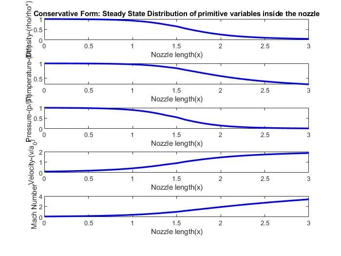
fig1
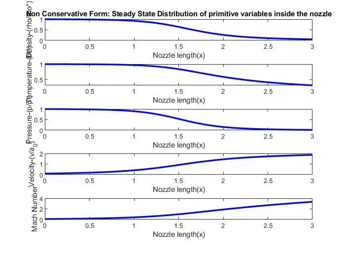
fig2
As seen on the graphs, the flow-field variables have a smooth transition from the subsonic region to the supersonic region of the nozzle.
B-Time-wise variation of primitive variables
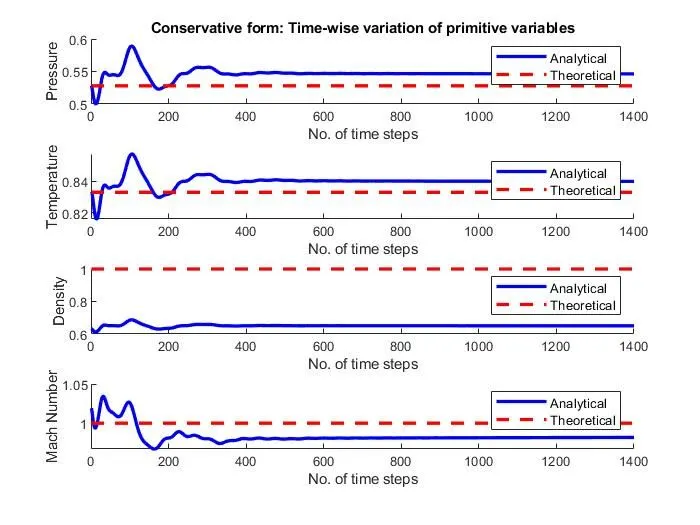
fig3
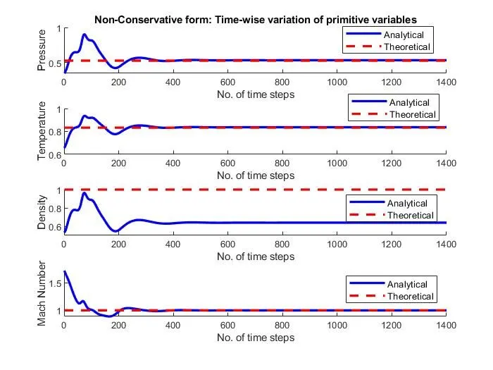
fig4
The pressure, temperature, density, velocity and the Mach number are plotted versus the number of time steps which ends at time step 1400. In the case of non-conservative form, one can notice through the four graphs that the largest changes take place at early times after which the final steady-state value is approached for each flow field variable. We assist to the concept of rubber band effect which means that at the early times, the rubber band is stretched tightly and therefore the flow-field variables are driven by a stronger potential and hence change rapidly. At later times, as the steady-state is approached the rubber band is less stretched. It becomes more relaxed and the changes become much smaller with time. Since the analysis is for an inviscid fluid, one can note that no artificial viscosity has been added as it is not needed.
C-Scaled residuals
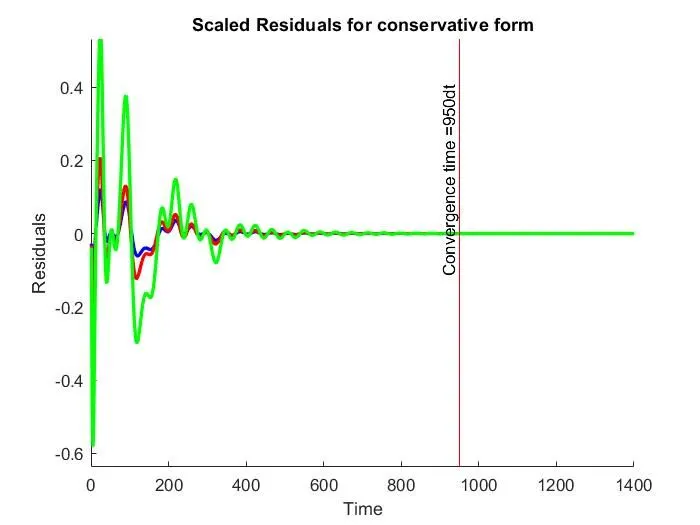
fig5
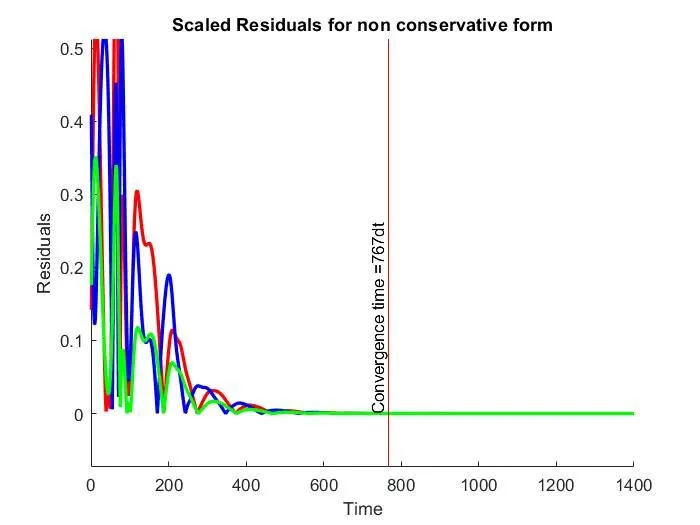
fig6
These graphs show the timewise variation of the absolute values of the time derivatives of non-dimensional density, velocity and temperature at the nozzle throat. We can see that at early times, there are considerable oscillations. This is because the time derivatives are large and they oscillate in value. Such oscillations let us say that there are unsteady compression and expansion waves propagation through the nozzle during the transient process.
At later times, we can see that the magnitudes drop sharply from a range of more than 0.5 to almost zeros over a span of 600-time steps. This happens because the derivatives rapidly grow small. From that point, we can notice that the values of the time derivatives plateau. Since these values are small and approach zero, we conclude that the numerical solution has arrived the steady state solution. Such conclusion is confirmed by the convergence point of the solution which appears to be at the position corresponding to 767-time steps.
D- Instantaneous mass flow rate at different time steps
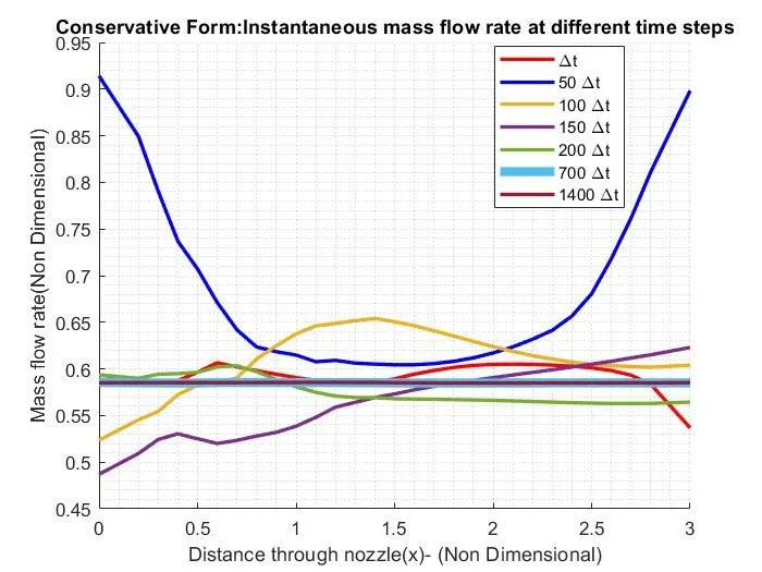
fig7
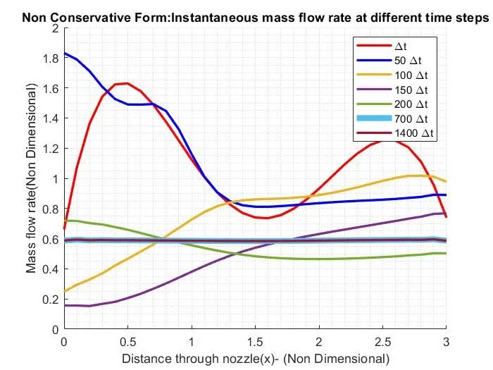
fig8
The mechanics of the timewise variation of the flow and its approach to the steady state is provided by the mass flow variations shown in the above figures.
The non-dimensional mass flow is as a function of non-dimensional distance through the nozzle. Seven different curves can be seen, each for a different time step during the course of the time-marching procedure. The one in red colour pertains to the starting point which corresponds to the initial conditions. Now, on the graph we can see that after 50-time step, the mass flow has changed considerably and it is shown by the curve labelled 50∆t. It can be also observed that after 100-time steps (100∆t), the mass flow distribution has changed radically. From there, the mass flow variation starts flopping (150∆t) around inside the nozzle due to the transient variation of the flow-field variables. However, after 200-time steps (200∆t), the mass flow distribution is beginning to settle down and after 700-time steps (700∆t), the mass flow distribution is a straight, horizontal line across the graph. This is confirmed by looking at the curves (700∆t) and (1400∆t) which are coincident. This means that the mass flow has converged to constant, steady-state value throughout the nozzle.
Before moving forward, let us discuss the results obtained for conservation form.
In fact, the steady state results obtained from the time-marching solution of the governing equations in conservation form are essentially the same as those obtained using the non-conservation form with a few slight, but notable difference. A comparative look to the first two figures allows us to note some little discrepancies. We conclude that, for all practical purposes, both forms of the governing equations give the same results.
However, we will highlight some of these discrepancies in the following section.
E- Mass flow rates comparison
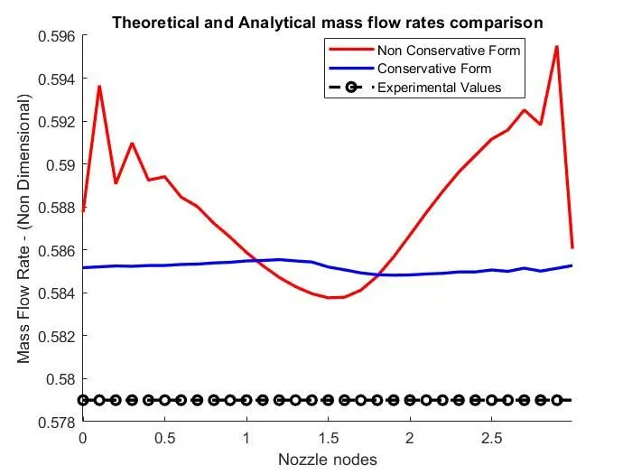
The most dramatic difference is in the mass flow distribution. The figure above shows the comparison of the mass flow distribution obtained in conservation form with the corresponding results in non-conservation form of the governing equations.
These curves show that the mass flow rate distribution in case of conservative form is smoother, uniform and much closer to the analytical solution as compared to non-conservative mass flow rate distribution. The last case shows an irregular distribution along the nozzle length. This urge to say that the steady-state mass flow distribution predicted by the conservation form of the equations is much more satisfactory than that obtained from the non-conservation form and also it does a better job of preserving mass throughout the flow field.
- Grid dependency test
The objective by running such test is to know if our solution is sensitive to the number of grid points. Since the results discussed above were obtained for a number of nodes N = 31, we have conducted a new analysis by doubling N this time; means N = 61. The
The table below compares the steady state results for density, temperature, pressure ratios and Mach numbers at the throat for both cases using 31 and 61 grid points.
|
Cases |
Number of nodes |
Density |
Temperature |
Pressure |
Mach number |
Time steps for convergence |
|
Non conservative form |
31 |
0.639 |
0.836 |
0.534 |
0.999 |
765 |
|
61 |
0.637 |
0.835 |
0.533 |
0.9997 |
1361 |
|
|
Conservative form |
31 |
0.650 |
0.840 |
0.546 |
0.982 |
950 |
|
61 |
0.638 |
0.835 |
0.533 |
0.999 |
1009 |
|
|
Exact analytical solution |
0.634 |
0.833 |
0.528 |
1.000 |
NA |
|
As it can be seen in the table, the accuracy is considerably increased in conservative form whereas it is increased by a small margin in case of non-conservative form. By comparing these values to the exact analytical results, we can note that although doubling the number of grid points did improve the numerical solution, it did so only marginally. Such case remains true for other parts of the nozzle. This means that the two numerical solutions are essentially the same; hence we can conclude that our original calculations using 31 grid points is essentially grid-independent. One more precision is that this grid independent solution does not agree exactly with the analytical results but it is certainly close enough.
As for the last column of the table, we can see that the non-conservative form has achieved the convergence in fewer time steps in case 31grid point. But the opposite happens when the grid points are increased to 61.
Conclusion
In essence, we applied both the conservation and non-conservation forms for solutions of the subsonic-supersonic isentropic nozzle flow and compared the results. For all practical purposes, the results are the same except that the conservation form yields a slightly better mass flow distribution. In other words, there is no superiority in either form of governing equation as far as the accuracy is concerned. The non-conservation form leads to smaller residuals and in the sense that the amount by which the residuals decay is often used as an index of quality of the numerical algorithm, the non-conservation form does a better job. However, there are cases where the need to use only one form of the governing equations is essential and such cases could be investigated further.
REFERENCES:
- https://www.grc.nasa.gov/www/k-12/airplane/nozzled.html
- https://www.grc.nasa.gov/www/k-12/airplane/isentrop.html
- John Anderson, Jr., COMPUTATIONAL FLUID DYNAMICS The Basics with Applications