Solving second order ODEs Using Python

AIM: To write a Python program which solves the equation of motion of a simple pendulum with damping.

OBJECTIVE:

• To learn how to solve an Ordinary Differential Equation (ODE) using Python
• To solve ODE of a simple pendulum that represents its equation of motion
• To simulate the pendulum motion
• Understand the importance behind motion study of a simple pendulum

Problem Statement

In Engineering, ODE is used to describe the transient behavior of a system. A simple example is a pendulum

The way the pendulum moves depends on the Newtons second law. When this law is written down, we get a second order Ordinary Differential Equation that describes the position of the "ball" w.r.t time.

Similarly, there are hundreds of ODEs that describe key phenomena and if you have the ability to solve these equations then you will be able to simulate any of theses systems.

Your objective is to write a program that solves the following ODE. This ODE represents the equation of motion of a simple pendulum with damping

In the above equation,

g = gravity in m/s2,

L = length of the pendulum in m,

m = mass of the ball in kg,

b=damping coefficient.

Write a program in Python that will simulate the pendulum motion, just like the one shown in the start of this challenge.

use,

L=1 metre,

m=1 kg,

b=0.05.

g=9.81 m/s2.

Simulate the motion between 0-20 sec, for angular displacement=0,angular velocity=3 rad/sec at time t=0.

When you do this you will get the position of the pendulum as a function of time. Use this information to animate the motion of the pendulum, as shown in the below figure.

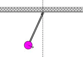
Your animation does not have to look exactly like this and here is the logic.

• For each value in time
• Create an image that represents the position of the pendulum
• You can assume the length of the string and the size of the ball
• Use the marker command to create a sphere
• One end of the pendulum is fixed
• The other end moves according to the solution of the ODE you had solved.
• If you are using using Matlab, use the movie command create an animation
• If you are using Octave you need to generate images first and then stitch them to form the animation

Theory:

An ordinary differential equation (ODE) is a differential equation containing one or more functions of one independent variable and the derivatives of those functions.

The ordinary differential equation under question here represents the equation of motion of a simple pendulum.

In fact, a simple pendulum consists of a mass m hanging from a string of length L and fixed at a pivot point P. So, in case it is tilted to an initial angle and released, the pendulum will swing back and forth with a periodic motion.

It lies on Newton’s second law and its study enables us to describe the simple harmonic motion or the theory of all oscillations.

Scientifically, pendulum finds its application in time-keeping even if nowadays it is getting substituted by atomic vibrations for the most accurate clocks. It is also used in the measurement of the acceleration due to gravity and also can be used the spinning of then earth.

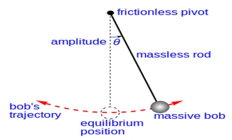
EQUATION USED:

• `(d^2 θ)/dt^2 + b/m ( dθ)/dt + g/L sin⁡θ = 0` where

g is the gravity in m/s^2

L is the length of the pendulum in m

m is the mass of the ball in kg

b is the damping coefficient

In order to write the Python program, the above equation is solved as following:

• Firstly, we substitute `θ= θ_1`

`(dθ)/dt= (dθ_1)/dt`

• `(dθ_1)/dt= θ_2` (1st ODE)

• `(d^2 θ)/dt^2 = (d^2 θ_1)/dt^2 = d/dt ((dθ_1)/dt)= d/dt(θ_2)`

• By rewriting the main equation we get

`(dθ_2)/dt+ b/m θ_2+ g/L sin⁡θ_1 =0` `⇒` `(dθ_2)/dt= - b/m θ_2- g/L sin⁡θ_1` (2^nd ODE)

By putting the above two ODEs in the matrix form we get:

`d/dt [θ_1@θ_2 ]= [θ_2@-(b/m) θ_2-(g/L )sin⁡θ_1 ]`

DETAILS:

Programming language used: Python

Concepts used: Ordinary Differential Equation, Simple pendulum, damping coefficient, Newton second Law.

Brief overview: This program in order to run and give the expected results, takes a help of a library that is "odeint library'. This library provides anumber of algorithms to solve initial value problems of ODEs. The focus of the library are explicit methods, although some implicit routines are also available. Odeint is written in C++ and uses modern programming techniques such as generic programming and other template metaprogramming to ensure high flexibility at optimal performance.

Loop used: For Loop

PROGRAAM AND STEPWISE EXPLANATION:

MAIN PROGRAM:

import numpy as np 
from scipy.integrate import odeint
import matplotlib.pyplot as plt
import math


#function that returns dz/dt

def model(theta,t,b,g,l,m):

	theta1 = theta[0]
	theta2 = theta[1]
	dtheta1_dt = theta2
	dtheta2_dt = -(b/m)*theta2-(g/l)*math.sin(theta1)
	dtheta_dt = [dtheta1_dt, dtheta2_dt]
	return dtheta_dt


b=0.05 # Damping Coefficient 
g=9.81 #Gravity in m/s^2
l=1 # Length in metre
m=1 # MAss in Kg 

#initial condition

theta_0 = [0,5]

#time points 
t = np.linspace(0,10,150)

#solve ODE

theta  = odeint(model,theta_0,t,args = (b,g,l,m))


#plot results

plt.plot(t,theta[:,0],'b-',label=r'$frac{dtheta_1}{dt}=theta2$')
plt.plot(t,theta[:,1],'r--',label=r'$frac{dtheta2}{dt}=-frac{b}{m}theta_2-frac{g}{L}sintheta_1$')
plt.ylabel('plot')
plt.xlabel('time')
plt.legend(loc='best')
plt.show()



x0 = 0
y0 = 0

alpha = theta[:,0]

ct = 1

for i in alpha:
	x1 = x0 + (l*math.sin(i))
	y1 = y0 - (l*math.cos(i))
	ct = ct + 1
	filename = str(ct) + '.png'


	plt.figure()
	plt.plot([-1,1],[0,0],'b-',linewidth=2)
	plt.plot([x0,x1],[y0,y1])
	plt.plot(x1,y1,'o', markersize = 20)
	plt.xlim([-2,2])
	plt.ylim([-2,2])
	plt.title('Simple Pendulum')
	plt.savefig(filename)

STEPWISE EXPLANATION OF THE PROGRAM

The first part of this about importing the diffferent libraries. Thus, the "numpy" library is imported as np and from "scipy.integrate" the "odeint" library is imported for integration. The "matplotlib.pyplot" library is also imported as plt and the "math" module is also imported.

After that comes the second part of the program which is about the function definition. The function "model" is defined which let us compute the first and second ODE staated above under equation session. The next part is about the definition of input variables. The damping coefficient, gravity, the pendulum length, the displacement and velocity, time as well as the mass are defined. Then the "odeint" library is called to integrate the "model" function.

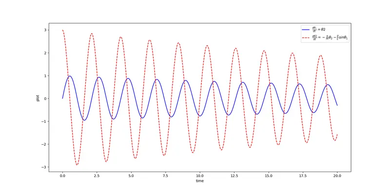
The fourth part of the program deal with plotting the two simplified ODEs using "plt" and 'plot' command. Plotting is done and legend is shown using 'legend' command.

In the fifth part of this program, the code deals with the creation of pendulum anaimation. The initial position of the pendulum rod is defined; then a counter is also defined which will let us create and store each image corresponding to each position of the pendulum. Under a for loop, each position of the pendulum is computed and stored as an image; those images which will be stiched together to give a full animation. After that, the pendulum is ploted using "markersize" command to create the mass at the end of the pendulum rod. A title is given to the plot using "title" command.

This marks the end of our program.

OUTPUT:

The simulation of simple pendulum motion can be consulted through the link belokw: