Simulation of a 2-DOF Robotic Arm using MATLAB Scripting
AIM:
- To write a program in MATLAB to simulate 2-D, 2-R forward kinematics of a 2 D.O.F. Robotic Arm.
- To also create an animation file of the simulation of the plots depicting the forward kinematics of the Robotic arm.
GOVERNING EQUATIONS AND RELEVANT THEORY:
- A robotic arm is a type of mechanical arm, usually programmable, with similar functions to a human arm; the arm may be the sum total of the mechanism or may be part of a more complex robot. The links of such a manipulator are connected by joints allowing either rotational motion (such as in an articulated robot) or translational (linear) displacement. The links of the manipulator can be considered to form a kinematic chain.
- Link: The word Link is used to designate a machine part or a component of a mechanism. It is assumed to be completely rigid. It is also referred to as a Kinematic Link.
- Kinematic Pair: When two links connect with each other, they are said to form a kinematic pair.
- Degrees of Freedom:
- Degree of Freedom of a body: An unconstrained rigid body moving in space can have the following independent motions:
- Translational motions along any 3 mutually perpendicular axes x, y and z.
- Rotational motions about the x, y and z axes.
- Degree of Freedom of a body: An unconstrained rigid body moving in space can have the following independent motions:
Thus a rigid body possesses 6 Degrees of freedom.
- Degree of Freedom of a pair: The connection of a link with another imposes certain constraints on their relative motion. The number of restraints can never be 0 (joint is disconnected) or 6 (joint becomes solid).
Degree of Freedom of a pair is defined as the number of independent relative motions, both translational and rotational, a pair can have.
Degrees of Freedom of a pair= 6-(Number of restraints)
Forward Kinematics: Forward kinematics refers to the use of kinematic equations of robot to compute the position of the end-effector from specified values for the joint parameters. Given a kinematic chain composed of links and joints with multiple degree of freedom, finding the position and orientation of the end-effector in the operational workspace when all the joint parameters are known. This is called FORWARD KINEMATICS.
OBJECTIVES OF THE PROJECT:
For my report, I will study the forward kinematics of a simple robotic arm as shown below:
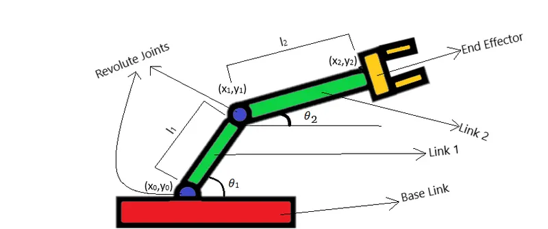
Robotic Arm
The forward kinematics of the above mechanism will be studied in a 2-D Cartesian plane.
The term 2-R means that the kinematic chain has two Revolute Joints.
As evident from the figure, the robotic arm has 3 links:
- A Base link which is a stationary platform and is also called the frame. It acts as a frame of reference for the other links i.e. motion for all other linkages will be measured w.r.t. to this link.
- Link 1 which is attached to the base link via a revolute joint.
- Link 2 which is attached to Link 1 via a revolute joint.
The Degree of Freedom of the above mechanism can be found out using the Kurtzback’s criterion:
DOF = 3(N-1)-2J-H
DOF = Degrees of Freedom.
N = No. of Links in the mechanism.
J = No. of Binary Joints in the mechanism
H=No. of Higher pairs in the mechanism.
In the above figure, the number of links are 3(Base link, Link 1 and Link 2), number of binary joints are 2(2 revolute joints) and number of higher pairs are 0.
Therefore DOF of the mechanism= 3*(3-1) – (2*2) – 0 = 6 – 4 = 2.
There is a revolute joint connecting the Base link and Link 1. The Base link is fixed. The Link 1 revolves about the revolute joint (connecting Link 1 and Base Link) in a 2D Cartesian plane and the range of rotation is 0 0 to 1800.
There is another revolute joint connecting Link 1 and Link 2. The Link 2 is also free to rotate about the revolute joint (connecting Link 2 and Link 1).
In order to study the Forward Kinematics of the robotic arm, we need to find the positions of the extreme ends of the links (Link 1 and Link 2). This can be done by some basic trigonometric calculations.
Let us consider the Link 1 first:
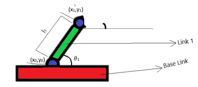
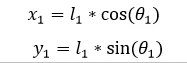
Link 1 can only rotate about the revolute joint connecting the Base Link and Link 1. The base Link remains fixed. If we consider the point where Link 1 meets the Base Link as origin i.e. assigning (x0, y0) = (0, 0) then co-ordinates of the other end of the Link 1 w.r.t. the revolute joint(joining Link 1 and Base Link) can be given by the following equation:
Now considering the Link 2 whose one extreme end is connected to Link 1 via a revolute joint and the other end connected to the end-effector.
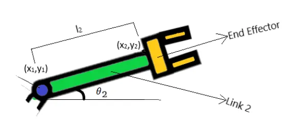
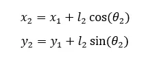
Link 2 will also revolve about the revolute joint (joining the Link 2 and Link 1). Therefore co-ordinates of the end effector (the end of Link 2 not attached to the revolute joint) w.r.t. to revolute joint (joining Link 1 and Link 2) is as follows:

Therefore the co-ordinates of the end-effector (the end of Link 2 not attached to the revolute joint) w.r.t. to revolute joint (joining the Base Link and Link 1) is as follows:
BODY OF THE CONTENT:
- Programming Language used: MATLAB.
- My code for simulating forward kinematics of a 2 D.O.F., 2-R Robotic Arm in a 2-D plane:
clear               %(clears the previous variables and their intialised values if any.)
close all           %(closes all the output windows of MATLAB if any.)
clc                 %(clears all the syntax and code previously written if any.)

%Inputs:
l1=1;               %(Initialised a variable 'l1'(signifies Link 1 dimension) with a value of 1)
l2=0.5;             %(Initialised a variable 'l2'(signifies Link 2 dimension) with a value of 0.5)
theta1=linspace(0,90,10);      %(Initialised a variable 'theta1'(signifies Link 1 angle w.r.t. horizontal axis) with 10 equally spaced values starting from 0 and ending at 90)
theta2=linspace(0,90,10);      %(Initialised a variable 'theta2'(signifies Link 2 angle w.r.t. horizontal axis) with 10 equally spaced values starting from 0 and ending at 90)
ct=0;                          %(Initialised a variable 'ct' with a value of 0)

for i=1:length(theta1)         %(Command to run the following contents inside this for loop 10 times)
    THETA1=theta1(i);          %(Initialised a variable 'THETA1' to take the value of theta1 according to the corrsponding values of 'i')

    for j=1:length(theta2)      %(Command to run the following contents inside this for loop 10 times)
        THETA2=theta2(j);       %(Initialised a variable 'THETA2' to take the value of theta1 according to the corrsponding values of 'j')

        %Defining the co-ordinates of the links:
        x0=0;                   %(Initialised the x-co-ordinate of the extreme end(connected to Base Link) of Link 1 to '0')
        y0=0;                   %(Initialised the y-co-ordinate of the extreme end(connected to Base Link) of Link 1 to '0')
        x1=l1*cosd(THETA1);     %(Initialised the x-co-ordinate of the extreme end(connected to Link 2) of Link 1 to take the value according to term in the R.H.S. of the relation)
        y1=l1*sind(THETA1);     %(Initialised the y-co-ordinate of the extreme end(connected to Link 2) of Link 1 to take the value according to term in the R.H.S. of the relation)

        x2=x1+(l2*cosd(THETA2));    %(Initialised the x-co-ordinate of the extreme end(connected to end effector) of Link 2 to take the value according to term in the R.H.S. of the relation)
        y2=y1+(l2*sind(THETA2));    %(Initialised the x-co-ordinate of the extreme end(connected to end effector) of Link 2 to take the value according to term in the R.H.S. of the relation)

        %Plotting:
        plot([x0 x1],[y0 y1],[x1 x2],[y1 y2],'linewidth',3)     %(Command to plot a line between (x0,yo) and (x1,y1) and from (x1,y1) to (x2,y2) and also setting the width of the lines to 3 units)
        axis([-1 2 0 1.5])              %(Setting the axis linits from -1 to 2 units in the x-axis and from 0 to 1.5 in the y-axis)
        pause(0.03)                     %(Setting a time gap of 0.03 time units between every consecutive plots.)
        ct=ct+1;                        %(Incrementing the counter loop variable 'ct' by 1 every time the loop runs.)

        %Labelling of axes of plots:
        xlabel('x-axis');               %(Labelling the x-axis of the plot as 'x-axis')
        ylabel('y-axis');               %(Labelling the y-axis of the plot as 'y-axis')

        %Inserting legends and title into the plots:
        legend('Link 1','Link 2');          %(Indicating the plot made by joining (x0,yo) to (x1,y1) as Link 1 and indicating the plot made by joining (x1,y1) to (x2,y2) as Link 2)
        title(['\theta_{1}=',num2str(THETA1),' and \theta_{2}=',num2str(THETA2)])       %(Adding a title on the top of the graph where θ1 and θ2 values are displayed for every corresponding position of Link 1 and Link 2)

        M(ct)=getframe(gcf);        %(Command to capture images/frames of plots for every single unique positions of Link 1 and Link 2 and assigning them to a variable 'M')

    end

end

%Creating a video file which shows the simulations of frames captured:
movie(M)                %(movie(M) plays the movie frames in array M once)
videofile=VideoWriter('forward_kinematics.avi','Uncompressed AVI');     %(Using a VideoWriter object to create a video file from the array M and assigning it to a variable named 'videofile')
open(videofile)                 %(Command to open a file assocoiated with 'videofile' for writing.)
writeVideo(videofile,M)         %(writeVideo command writes one or more movie frames typically returned by the getframe function)
close(videofile)                %(Command to close the video file assocoiated with 'videofile' to ensure that all data is written to the file.)
- The above code has been written in the Editor window of MATLAB.
- In MATLAB, anything written at a particular line starting with the special character '%' are comments for this programming language. The compiler skips anything that starts with '%' in a line while compiling and running the code.
- For the above case, I have used comments beside the code in each and every line to explain the functionality of that particular code.
- In the above code I have initialised 2 variables ‘l1’ and ‘l2’ with integer values where l1 and l2 represents the lengths of the link 1 and link 2 respectively.
- I have also initialised theta1(represents θ1)and theta2(represents θ2) with an array of integer values(in row matrix form) where it will take 10 equally spaced values and the initial value and final value for both theta1 and theta2 are 0 and 90 respectively.
- I have taken 2 ‘for’ loops where one ‘for’ loop is inside another ‘for’ loop.
- The outer ‘for’ loop will run the content inside it 10 times (signified by length(theta1)) as the number of values taken for theta1 taken is 10.The content inside the loop will run for every single value of θ1.
- The inner ‘for’ loop will also run the content inside it 10 times (signified by length (theta2)) for each theta1 value as the number of values taken for theta2 is 10.The content inside this loop will run for every single value of θ2 for every corresponding value of θ1.
- Within this inner ‘for’ loop the co-ordinates of the links are defined.
- The co-ordinates will be established every time the inner ‘for’ loop runs. The inner for loop will run for 10 X 10=100 times as there will be a 10 θ2 values for every θ1.
- After getting the θ2, θ1 values, we get the co-ordinates of the links via the equations.
- After getting the values of θ1 and θ2, I put a command to join the co-ordinates (found for various angles of θ1 and θ2).
- Thus plots for Link 1 and Link 2 are formed for various values of θ1 and θ2 are formed.
- After plotting the links we use the MATLAB functions like getframe, movie, VideoWriter, open, writeVideo and close to capture the frames of each distinct plot and use the frames to create a video/movie/simulation of the plots.
RESULTS: On running the code, I get an output like this:*Click on the following Link:*
https://drive.google.com/file/d/13D9ntAM2HYeKEy3sPTnjSkVRmIID0e14/view?usp=sharing
and additionally a mkv(Video File format) named ‘forwardkinematics.avi’ gets saved in the folder where the program file has been saved.
That file plays a video which shows the simulation of the forward kinematics of the Robotic arm:*Click on the following Link:*
https://drive.google.com/file/d/1xzcUkXNoEhhui96JqxxgOLbKz7DdR43u/view?usp=sharing
ERRORS FACED WHILE PROGRAMMING:
- Error 1: For arrays in MATLAB indexing starts from 1 unlike in C/C++ programs where indexing starts from 0. Therefore for invoking the very first value of an array we need to make sure that index value is 1 and not zero.
For example in my program, I had initialised the counter loop variable as 0 outside the for loop and while using the the getframe command to collect the images of the plots formed, the first index for array variable M was put to 0 as I had not incremented the counter loop variable ‘ct’ by 1 before using the function. Instead I had incremented the counter loop variable ‘ct’ by 1 after using the getframe function where the first index value of M was set to 0.Therefore I was shown an error as follows:
Mistake made and error displayed:
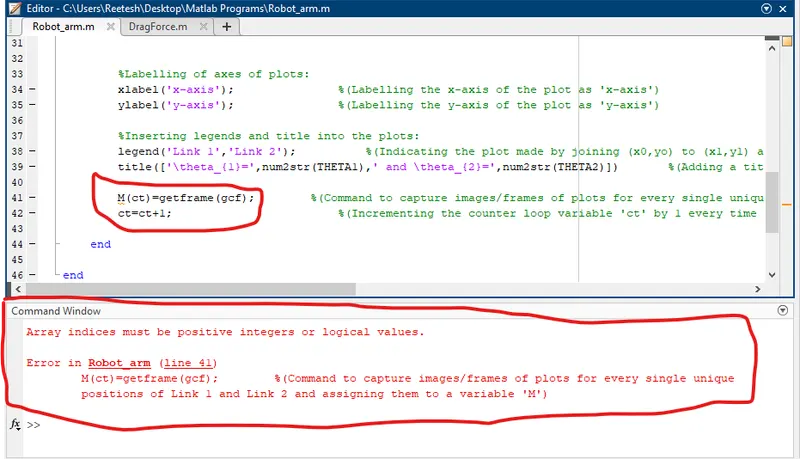
The error thrown by MATLAB is shown in the command window.
Correction made: As shown in my main code, I have incremented the counter loop variable before using the getframe function.
- Error 2: Plotting outside the inner loop (the loop which takes into consideration all the values of θ2 for all corresponding values of θ1).
This won’t throw an error but the resultant plots formed are wrong. And the simulation formed will show Link 1 changing its position in accordance to θ1 value but the position of Link 2 in the simulation remains static. This happens because the inner loop gets executed first 9 times without any plotting and then plots the result of that loop (10th time which is the last time the inner loop runs) for any particular loop run of the outer ‘for’ loop and hence plots the result of the 10th (last) loop run of the inner ‘for’ loop (always at 90 degrees) for all loop runs of the outer ‘for’ loop.
Mistake Made:
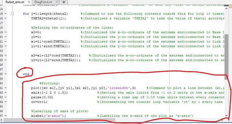
As shown in the image, the plotting has been done outside the inner ‘for’ loop.
Output due to this error:*Click on the following Link:*
https://drive.google.com/file/d/1nR0bc_JvMWIOpHg8BGPLfcDtqU-loNRN/view?usp=sharing
Correction made: Plotting done within the inner ‘for’ loop as shown in the main code.
- Error 3: Wrong MATLAB syntax for plotting of graphs:
In general we identify a point in a graph by it’s x co-ordinate and y-co-ordinate and represent that point as (x, y) where x and y are the x co-ordinate and y-co-ordinate of that point respectively. Hence in order to join any two points in a graph, it’s representation using pen & paper is generally done by join (x0, y0) and (x1, y1). There is a huge chance that a MATLAB programmer will pass the syntax as:
plot ([x0,y0],[x1 y1])
to join these two points.
However this syntax in MATLAB is wrong as we need to write x- co-ordinates of both points first in square brackets and then write the y- co-ordinates of both the points in square brackets.
Mistake made:
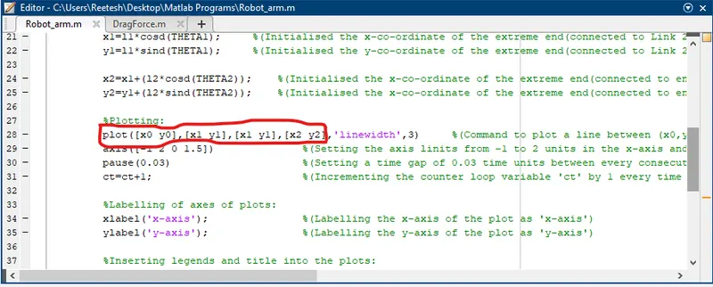
Output due to this mistake: We get a plot and simulation that doesn’t represent the kind of output I was expecting:*Click on the following Link:*
https://drive.google.com/file/d/1mGbcGpNmph6U3-mDNg_ysqE2M9tTsV4l/view?usp=sharing
Correction made: Put the right syntax for plotting as per MATLAB as shown in my main code. Command should be:
plot([x0 x1],[y0 y1],[x1 x2],[y1 y2]).
- Error 4:Different code for calculating sin and cos values in radians and in degrees:
According to MATLAB, the syntax for finding out trigonometric functions of integers is different for angles in radians and degrees.
Syntax for finding trigonometric function values of angles in radians:
sin(angle),cos(angle),tan(angle),etc.
Syntax for finding trigonometric function values of angles in degrees:
sind(angle),cosd(angle),tand(angle),etc.
However I made put the syntax for finding trigonometric functions of angles in radians while in actual I wanted to find the values of trigonometric functions of angles in degrees.
Mistake made:
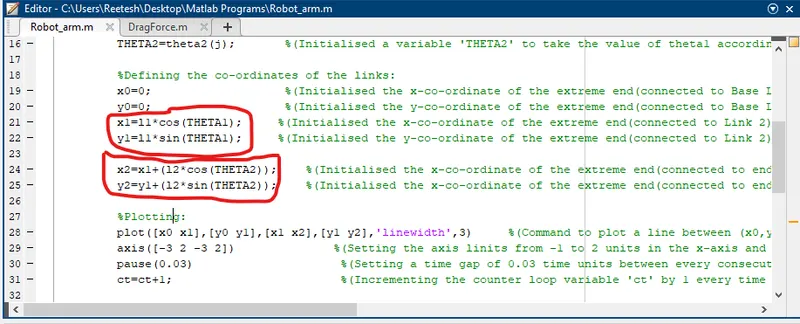
Note: I have changed the axis limits here to show how this particular error affects the simulation.
Output due to this error: We get plots and their simulation and it’s not the kind of output I was expecting:*Click on the following Link:*
https://drive.google.com/file/d/1QZrU8QKHYRxUsFHFJhHmm3Ej71nHBkgW/view?usp=sharing
Correction made: Instead of putting the syntax for calculating trigonometric functions in radians, I put the syntax for calculating trigonometric function in degrees.
x1=l1*cosd(THETA1);
Y1=l1*sind(THETA1);
x2=x1+(l2*cosd(THETA1));
y2=y1+(l2*sind(THETA1));
Error 5: While using a MATLAB function named VideoWriter I wrote Videowriter instead of VideoWriter. It threw an error on running the program as MATLAB is a case sensitive programming language and i.e. the if the same name written in ways such that if at least one of the letters differ in letter case(in 1 case it is uppercase and in another case, it is lowercase) then the two names are considered to be distinct.
In my mistake, I wrote the ‘W’ of VideoWriter function in lower case instead of uppercase.
Mistake made (see Editor Window) and the error thrown (see Command Window):
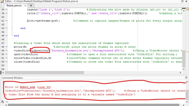
Correction made: Changed the ‘W’ of VideoWriter from ‘w’ to ‘W’.
CONCLUSION:
- MATLAB is a great programming language and a platform to understand, analyse, simulate dynamics of mechanical body or it’s components.
- Robotic arm is one such mechanical body where we can use MATLAB to simulate its forward kinematics.
- We can also analyse the kinematics of each component of a Robotic arm and make required conclusions necessary for designing a robotic arm.
- Yesterday’s engineer spent a major portion of his or her time substituting values into the formulas and obtaining numerical results. However, formula manipulations and number crunching are now being left mainly to computers. Tomorrow’s engineer will need a clear understanding and a firm grasp of the basic principles so that he or she can understand even the most complex problems, formulate them, and interpret the results. MATLAB is one such fundamental tool which aids and will continue to aid tomorrow’s engineers.