DC Motor Mathematical Modelling using Simulink

IM:

Develop Simulink Model of a DC Motor based on information available below. Find Requirement Document attached herewith. Expected Result files are the Simulink model & an init file.

Problem Statement:

DC Motor Problem Statement

A common actuator in control systems is the DC motor. It directly provides rotary motion and, coupled with wheels or drums and cables, can provide translational motion. The electric circuit of the armature and the free-body diagram of the rotor are shown in the following figure:

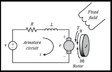
We will assume that the input of the system is the voltage source (𝑉) applied to the motor's armature, while the output is the rotational speed of the shaft 𝜃̇. The rotor and shaft are assumed to be rigid. We further assume a viscous friction model, that is, the friction torque is proportional to shaft angular velocity.

The physical parameters for our example are:

(J) moment of inertia of the rotor 0.01 kg.m^2

(b) motor viscous friction constant 0.1 N.m.s

(Ke) electromotive force constant 0.01 V/rad/sec

(Kt) motor torque constant 0.01 N.m/Amp

(R) electric resistance 1 Ohm

(L) electric inductance 0.5 H

In general, the torque generated by a DC motor is proportional to the armature current and the strength of the magnetic field. In this problem, we will assume that the magnetic field is constant and, therefore, that the motor torque is proportional to only the armature current 𝑖 by a constant factor 𝐾𝑡 as shown in the equation below. This is referred to as an armature-controlled motor.

𝑇= 𝐾𝑡𝑖

The back emf, 𝑒 is proportional to the angular velocity of the shaft by a constant factor

𝐾𝑒 𝑒= 𝐾𝑒𝜃̇

Create an init file in MATLAB to declare & initialize the input values. Model input is Voltage & Output is Rotor Speed

(Note: Simulink has to modelled with respect to the differential calculus equations, creation of simulink model using Simscape environment ,accordingly marks will be deducted ).

SOLUTION TO THE OBJECTIVE:

Introduction to DC Motor: The Actuator used in motor Controllers is the DC Motor. These DC Motors convert Electrical Energy to Mechanical Energy using Direct Current (DC).

Working Principle: A DC Machine (motor/generator) works on the principle of Lorentz’s Law which states that a current carrying conductor placed in an electromagnetic field (magnetic and electric field) experience a force.

Fleming’s Left Hand Rule is used to obtain the direction of this force based on the Current and Magnetic Field Direction.

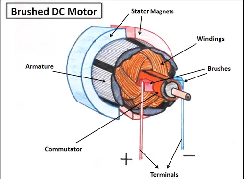
Brushed DC Motor

In the problem, the mathematical model of the DC Motor has to be done as per the following assumptions:

Assumptions:

• The Rotor and Shaft are assumed to be rigid. Note that neither the Rotor is rigidly attached to the shaft nor the shaft is attached rigidly attached in the motor.
• The Model is a Viscous Friction Model where the Frictional Torque is proportional to the Shaft Angular Velocity. The Relation between the Frictional Torque and the Angular Velocity is assumed to be as follows:

T_friction = b*(dθ/dt) = b*ω

Where b = Motor Viscous Friction Constant or the Damping Coefficient

θ = Angular Displacement of the Shaft/Rotor.

(dθ/dt) = ω = Angular Velocity of the Shaft/Rotor.

T_friction = Frictional Torque

• As per the Question, the Magnetic Field is constant. Therefore, the Torque generated by the DC Motor is proportional only to the Armature Current ‘i’ as per the following relation:

T_motor = K_ti

where T_motor = Motor Torque

K_t­­ = Motor Toque Constant

i = Armature Current

• As per the Question, the back emf ‘e’, is proportional to the angular velocity of the shaft/rotor by a constant factor K_e :

e = K_e (dθ/dt) = K_e ω

where (dθ/dt) = ω = Angular Velocity of the Shaft/Rotor

K_e = Constant Factor proportionating the back emf and the angular velocity.

Governing Equations:

According to Newton’s 2^nd Law of Rotation, if more than one torque acts on a rigid body about a fixed axis, then the sum of the torques equals the moment of inertia times the angular acceleration. Here the rigid body is the Rotor. According to the Information for the Model provided via Explanations, Assumptions and Diagram, Newton’s 2^nd Law can be applied on the Rotor according to the following relation:

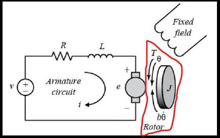
Newton's 2nd Law applied to the encircled part

T­­_net = J α = J (dω/dt) = J (d²θ/dt²).

T_net = J (d²θ/dt²) = Net Torque acting on the Rotor

T_net = J (d²θ/dt²) = T_motor – T_friction

T_net = J (d²θ/dt²) = (K_t i) – b(dθ/dt)

(d²θ/dt²) = (1/J) * [ (K_t i) – b(dθ/dt)] __________________________(a)

where T_net = Net External Torque on the Rotor

J = Moment of Inertia of the Rotor

α = (dω/dt) = (d²θ/dt²) = Angular Acceleration of the Rotor

T_motor = Motor Torque

T_{friction ­}= Frictonal Torque on the Rotor

K_t = Motor Torque Constant

i = Armature Current

b = Motor Viscous Friction Constant

ω = (dθ/dt) = Angular Velocity of the Rotor

θ = Angular Displacement of the Rotor

Now applying Kirchoff’s Law (KVL) to the Electrical Part of the Circuit in the Motor:

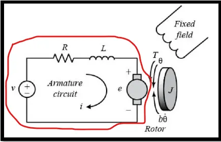
Kirchoff's Voltage Law (KVL) applied to the Encircled Part

Applied Input Voltage = Voltage Drops in the Circuit

Applied Input Voltage = (Voltage Drop due to Armature Resistance) + (Voltage Drop due to Inductance) + (Voltage Drop due to back emf)

V = iR_a + L(di/dt) + e

L(di/dt) = V – iR_a – e

(di/dt) = 1/L [V – iR_a – e] ­­­­

(di/dt) = 1/L [V – iR_a – K_e(dθ/dt)] __________________________________(b)

Equations (a) and (b) will be used to model the given System in Simulink.

Modelling:

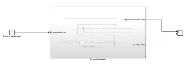
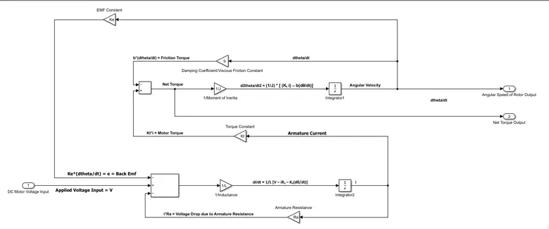
• Simulink Blocks used for implementing this model include Inport, Outport, Integrator, Add and Gain Blocks inside the DC Motor Subsystem (implemented by adding the Subsystem Block in the main System Window) and Constant Block + Scope Block outside the Subsystem in the Main System Window.
• The Blocks have been added and connected amongst each other so as to represent the equations (a) and (b) which represent the behaviour of the Model as mentioned in the problem statement.
• The Main Model is as follows:

• Equations (a) and (b) application implemented in the Subsystem Model. The Subsystem Model is as follows:

• In order to initialize the Unknown Constants in the Model, the Variables (as per defined in Simulink) are initialized in a new Script File the MATLAB Main Window.

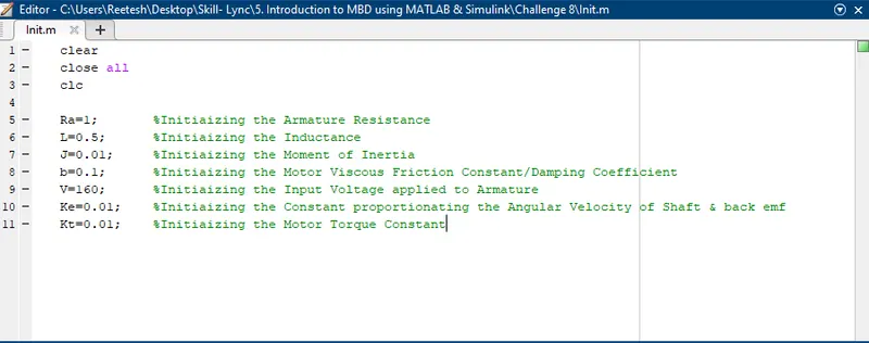
• After initializing the Variables in the New Script File, it is now run. After Running the Script File, the user may be prompted to save the File. It is to be noted that the Script File should be saved in the same Location which houses the Simulink Model File. After running the File, the variables along with their Values are loaded into the Workspace.

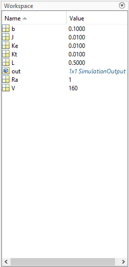
• Once the Variables and their values are loaded into the Workspace, the Simulink Model is run and the results are analysed in the Scope Block.

Result:

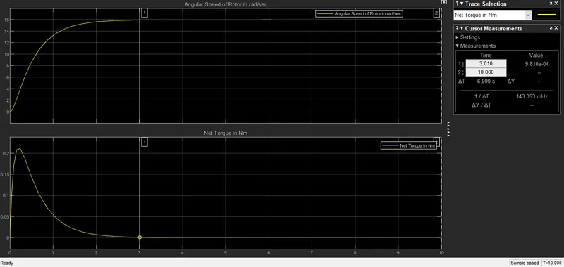
The Result in the Scope Block shows the Waveforms of the Net Torque and the Angular Velocity of the Rotor based on the values provided to the relevant parameters in the ‘init’ file.

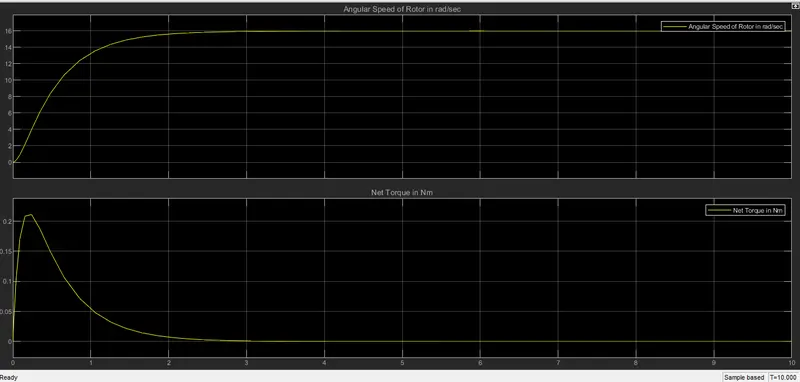
Based on the Result obtained, the following conclusions can be drawn:

• As the Rate of Increase of Angular Speed of the Rotor increases, the Net Torque increases.This is because T_net=J*(dω/dt) and as (dω/dt) increases, T_net increases.

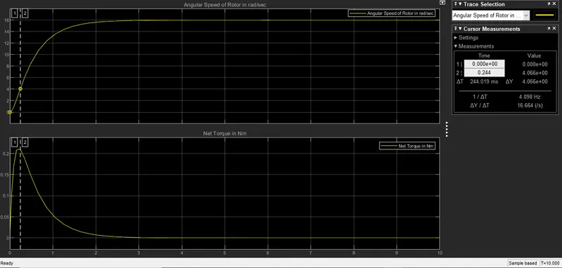
• As The Rate of Increase of the Angular Speed of the Rotor decreases, the Net Torque starts decreasing.This is because T_net=J*(dω/dt) and as (dω/dt) decreases, T_net decreases.

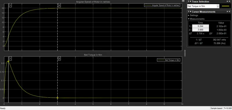
• As The Rate of Increase of the Angular Speed of the Rotor continues to decrease until the Angular Speed of the Rotor becomes constant, the Net Torque on the Rotor also continues to decrease and when the Angular Speed of the Rotor becomes Constant, the Net Torque becomes 0.This is because T_net=J*(dω/dt) and as ω becomes constant (dω/dt) becomes 0 , T_net also becomes 0.
• As long as the Angular Speed of the Rotor remains constant, the Net Torque on the Rotor remains 0.