Challenge

Genetic Algorithm Implementation using MATLAB Programming

RReetesh Nag23 Mar 2023

MATLAB

AIM:

To write a code in MATLAB to optimize the stalagmite function and find the global maxima of the function using the in-built ‘ga’ function of MATLAB.
Plotting the variation of optimal solutions against the independent variable(s).

GOVERNING EQUATIONS AND RELEVANT THEORY:

First, we have to optimize the stalagmite function which is given by:

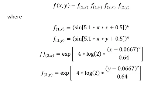
The above function is dependent on a given set of parameters/variables(x and y).
Optimization of a given function means finding out the best possible solution of a given function provided the solution satisfies all the constraints for the given function.
The process involves comparing various solutions of the function iteratively till an optimal/satisfactory solution is obtained.
There are various procedures for obtaining an optimal solution for a given function.
One such procedure is the Genetic Algorithm.
The Genetic Algorithm is based on Charles Darwin’s theory of Natural Evolution.
According to this theory of Natural Evolution, the fittest among a given population are selected to produce offspring(s) for the next generation.
In the world of Mathematics and Computers, the Genetic Algorithm functions in a way similar to the theory of Natural Evolution.
At each iteration, the algorithm does the following steps:
In the algorithm, a given radom population (values of independent variables) is taken as input. The algorithm then selects a set of independent variable values (parents) at random from the given population and their solutions are generated.
The algorithm then repeatedly modifies the population of individual solutions. These solutions will become the population for the next generation.
Over successive generations, the population evolves towards an optimal solution.
The algorithm makes use of Biological evolution rules like Selection, Crossover, and Mutation to create the next generation from the current population.

The Genetic Algorithm in MATLAB is implemented using an in-built MATLAB function named ‘ga’.
The ‘ga’ function is used to find out the global minima of a given function from each random sample of data points.
When ‘ga’ is implemented, MATLAB does the following:
- A random set of variable values is created and taken as the initial population for the algorithm to create individual solutions.
- The best possible solutions are selected among this population to give the next set of solutions for the next generation.
- This set of individual solutions becomes the population for the next generation and will be used to create a further new set of individual solutions.
- In this way, a sequence of new population is created.
- The algorithm keeps running until it reaches a termination point where one of the following conditions are satisfied:
  - Time Limit for the algorithm to run: A user can set up the time limit for which the algorithm can run.
  - Iteration Limit: A user can specify the number of generations/iterations for which the algorithm will keep computing the best possible solutions. Each iteration involves evaluating the best possible solutions from the best possible set of variables values taken from a population.
  - Tolerance Limit: A user can specify the tolerance within which the best-fit solutions of the function can vary. The algorithm runs until the average relative change in the fitness function value is less than the Function tolerance limit.

BODY OF THE CONTENT:

Programming language used: MATLAB.
Attached below is the code:

clear 
close all
clc

%Defining our search space:
x=linspace(0,0.6,150);
y=linspace(0,0.6,150);

%Defining number of generations:
num_case=50;


%Creating a 2-D mesh:
[xx, yy]=meshgrid(x,y);

%Evaluating the stalagmite function:
for i=1:length(xx)
    for j=1:length(yy)
        input_vector(1)=xx(i,j);
        input_vector(2)=yy(i,j);
        f(i,j)=stalagmite(input_vector);
    end
end

%Plotting the xx,yy and the corresponding 'f' value on a 3-D plot:
surfc(xx,yy,-f)
xlabel('x value')
ylabel('y value')
shading interp

[inputs, fvalmin]=ga(@stalagmite,2)
fvalmax=-fvalmin

%Study-1-Statistical behaviour:
tic
for i=1:num_case
    [inputs,foptmin(i)]=ga(@stalagmite,2);
    xopt(i)=inputs(1);
    yopt(i)=inputs(2);
    foptmax(i)=-foptmin(i);
end
Study1_time=toc;

figure(2)
subplot(2,1,1)
hold on
surfc(xx,yy,-f)
shading interp
plot3(xopt,yopt,foptmax,'marker','o','markersize',5,'markerfacecolor','r')
title('Unbounded inputs')
xlabel('x-values')
ylabel('y-values')
zlabel('Function-values')
subplot(2,1,2)
plot(foptmax,'Linewidth',2)
xlabel('Iterations')
ylabel('Function maximum')

%Study2:Statistical behaviour with upper & lower bounds:
tic
for i=1:num_case
    [inputs,foptmin(i)]=ga(@stalagmite,2,[],[],[],[],[0;0],[1;1]);
    xopt(i)=inputs(1);
    yopt(i)=inputs(2);
    foptmax(i)=-foptmin(i);    
end
Study2_time=toc;

figure(3)
subplot(2,1,1)
hold on
surfc(xx,yy,-f)
shading interp
plot3(xopt,yopt,foptmax,'marker','o','markersize',5,'markerfacecolor','r')
title('Bounded inputs')
xlabel('x-values')
ylabel('y-values')
zlabel('Function-values')
subplot(2,1,2)
plot(foptmax,'Linewidth',2)
xlabel('Iterations')
ylabel('Function maximum')


%Study3:Increasing Population Size:
options=optimoptions('ga');
options=optimoptions(options,'PopulationSize',350);

tic
for i=1:num_case
    [inputs, foptmin(i)]=ga(@stalagmite,2,[],[],[],[],[0;0],[1;1],[],[],options);
    xopt(i)=inputs(1);
    yopt(i)=inputs(2);
    foptmax(i)=-foptmin(i);
end

Study3_time=toc;

figure(4)
subplot(2,1,1)
hold on
surfc(xx,yy,-f)
shading interp
plot3(xopt,yopt,foptmax,'marker','o','markersize',5,'markerfacecolor','r')
title(['Bounded inputs with Population size=',num2str(options.PopulationSize)])
xlabel('x-values')
ylabel('y-values')
zlabel('Function-values')
subplot(2,1,2)
plot(foptmax,'Linewidth',2)
xlabel('Iterations')
ylabel('Function maximum')

Note that we need to find out the maxima of the stalagmite fitness function using the in-built ‘ga’ function.
‘ga’ function directly gives the value of possible minima(s) of the function.
In order to use ‘ga’ to get the maxima of the fitness function, we need to apply ‘ga’ on the mirror image(about the horizontal (x) axis) of the stalagmite function.
If the stalagmite function is given by f_xy, then in order to find the maxima of the function using ‘ga’, we need to apply ‘ga’ on –f_xy.
Thus the maxima of f_xy becomes minima of –f_xy and minima of f_xybecomes maxima of –f_xy.
First, I make a function file in which the stalagmite fitness function has been defined:

function [fxy]=stalagmite(input)

    x=input(1);
    y=input(2);
    f1x=(sin(5.1*pi*x+0.5)).^6;
    f1y=(sin(5.1*pi*y+0.5)).^6;
    f2x=exp((-4)*(log(2))*((x-0.0667)^2/0.64));
    f2y=exp((-4)*(log(2))*((y-0.0667)^2/0.64));
    fxy=-(f1x*f2x*f1y*f2y); 
end

Note that the original function has been multiplied with (-1) in order to obtain a global maxima using the ‘ga’ command in the main program file.

In the function file, I have written a code to define the stalagmite fitness function file where the function takes input of a 2-D vector where the 1^st element of the vector corresponds to the x-element (independent variable) and the 2^nd element of the vector corresponds to the y-element (independent variable) and the function returns the value of the function as a scalar.
Now, attached below is the code wherein I will call the stalagmite function for x-values and y-values.

%Defining our search space:
x=linspace(0,0.6,150);
y=linspace(0,0.6,150);

%Defining number of generations:
num_case=50;


%Creating a 2-D mesh:
[xx, yy]=meshgrid(x,y);

%Evaluating the stalagmite function:
for i=1:length(xx)
    for j=1:length(yy)
        input_vector(1)=xx(i,j);
        input_vector(2)=yy(i,j);
        f(i,j)=stalagmite(input_vector);
    end
end

%Plotting the xx,yy and the corresponding 'f' value on a 3-D plot:
surfc(xx,yy,-f)
xlabel('x value')
ylabel('y value')
shading interp

Note that that the value of function will be stored in the variable ‘f’ and the values of the function are computed with using the x and y values stored as vectors.
meshgrid function helps in the formation of matrices from which we can compute the function values for all possible combinations of x and y variable values.
Now, I will plot the function values along with their corresponding x and y value variables.
Attached below are the 3-D plots:

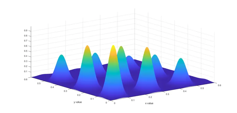
After all possible function values have been computed, it is now time to implement the genetic algorithm.
The genetic algorithm will be implemented for this function for 3 different cases, where each case corresponds to a unique syntax of the ‘ga’ function.
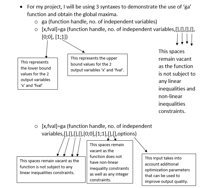
the ‘ga’ MATLAB function can be implemented using these following syntaxes:
- x= ga(function handle, nvars) finds a local unconstrained minimum, x, to the objective function declared as a function handle to be taken as input for implementing ‘ga’. ‘nvars’ is the dimension (number of design/independent variables) of objective function.
- x= ga(function handle, nvars ,A, b) finds a local minimum x to the objective function , subject to the linear inequalities A*x ≤ b. ga evaluates the matrix product A*x as if x is transposed (A*x').

x= ga(function handle, nvars, A, b, Aeq, beq) finds a local minimum x to the objective function, subject to the linear equalities Aeq*x = beq and A*x ≤ b. (Set A=[] and b=[] if no linear inequalities exist.) ga evaluates the matrix product Aeq*x as if x is transposed (Aeq*x').

x= ga(fun,nvars,A,b,Aeq,beq,lb,ub) defines a set of lower and upper bounds on the design variables, x, so that a solution is found in the range lb ≤ x ≤ ub. (Set Aeq=[] and beq=[] if no linear equalities exist.)

x= ga(fun,nvars,A,b,Aeq,beq,lb,ub,nonlcon) subjects the minimization to the constraints defined in nonlcon. The function nonlcon accepts x and returns vectors C and Ceq, representing the nonlinear inequalities and equalities respectively. ga minimizes the fun such that C(x) ≤ 0 and Ceq(x) = 0. (Set lb=[] and ub=[] if no bounds exist.)

x= ga(fun,nvars,A,b,Aeq,beq,lb,ub,nonlcon,options) minimizes with the default optimization parameters replaced by values in options. (Set nonlcon=[] if no nonlinear constraints exist.) Create options using optimoptions.

x= ga(fun,nvars,A,b,[],[],lb,ub,nonlcon,IntCon) or x = ga(fun,nvars,A,b,[],[],lb,ub,nonlcon,IntCon,options) requires that the variables listed in IntCon take integer values.
x= ga (problem) finds the minimum for problem, a structure described in problem.

[x, fval] = ga (___), for any previous input arguments, also returns fval, the value of the fitness function at x.

[x, fval, exitflag, output] = ga(___)also returns exitflag, an integer identifying the reason the algorithm terminated, and output, a structure that contains output from each generation and other information about the performance of the algorithm.

[x, fval, exitflag, output, population, scores] = ga(___) also returns a matrix population, whose rows are the final population, and a vector scores, the scores of the final population.

Case 1: Evaluating the global maxima of the stalagmite function when no constraints are given.
Attached below is the code:

%Study-1-Statistical behaviour:
tic
for i=1:num_case
    [inputs,foptmin(i)]=ga(@stalagmite,2);
    xopt(i)=inputs(1);
    yopt(i)=inputs(2);
    foptmax(i)=-foptmin(i);
end
Study1_time=toc;

figure(2)
subplot(2,1,1)
hold on
surfc(xx,yy,-f)
shading interp
plot3(xopt,yopt,foptmax,'marker','o','markersize',5,'markerfacecolor','r')
title('Unbounded inputs')
xlabel('x-values')
ylabel('y-values')
zlabel('Function-values')
subplot(2,1,2)
plot(foptmax,'Linewidth',2)
xlabel('Iterations')
ylabel('Function maximum')

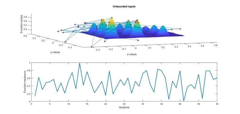
In this case, in the 1^st iteration, the ‘ga’ function takes 180 values from a random set of x and y values and produce the most optimal solutions from these 180 values.

In the 2^nd iteration, the solutions inherited from 1^st population become the population on which the ‘ga’ function will act and again produce new solutions.

Thus there will be 50 such iterations and each iteration will produce a minima. One of these minimas produced may or may not be the global minima. The x and y values corresponding to the fitness values obtained while implementing ‘ga’ may go beyond the domain of x and y values defined for computing the stalgmite function as there are no constraints involved. This is evident from the plots obtained.

Case 2: Evaluating the global maxima of the stalagmite function when upper and lower bounds for the functions have been defined.

Attached below is the code:

%Study2:Statistical behaviour with upper & lower bounds:
tic
for i=1:num_case
    [inputs,foptmin(i)]=ga(@stalagmite,2,[],[],[],[],[0;0],[1;1]);
    xopt(i)=inputs(1);
    yopt(i)=inputs(2);
    foptmax(i)=-foptmin(i);    
end
Study2_time=toc;

figure(3)
subplot(2,1,1)
hold on
surfc(xx,yy,-f)
shading interp
plot3(xopt,yopt,foptmax,'marker','o','markersize',5,'markerfacecolor','r')
title('Bounded inputs')
xlabel('x-values')
ylabel('y-values')
zlabel('Function-values')
subplot(2,1,2)
plot(foptmax,'Linewidth',2)
xlabel('Iterations')
ylabel('Function maximum')

In this case, similar to the previous case, the only thing extra done is adding the range for the output from the ‘ga’ algorithm.

In this case, the lower bound has been defined as 0 for both the inputs and the function value and the upper bound has been defined as 1 for both inputs and the function values.

Doing this small addition has led to give a more accurate outputs compared to the previous case, where the outputs were all over the place. Attached below are the plots obtained:

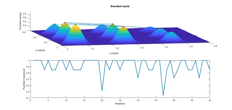
View 1.

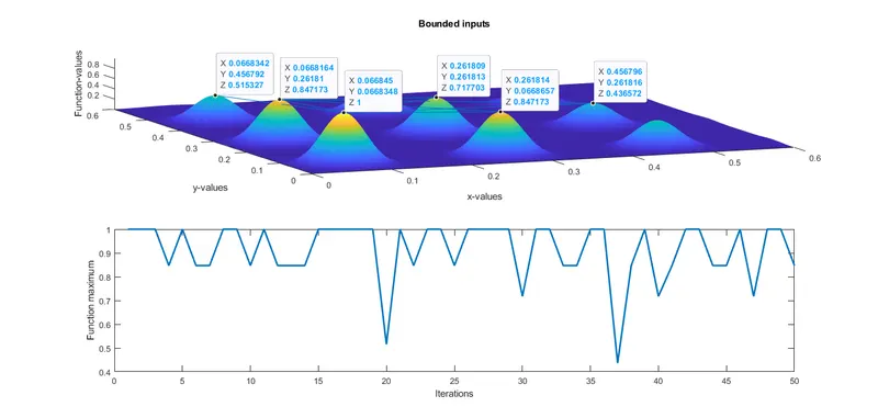
View 2

As can be seen, the independent variables and the values of the function obtained lie in the range [0, 1]

Case 3: Evaluating the global maxima when the population size for the algorithm is defined in ‘ga’ function definition

Attached below is the code:

%Study3:Increasing Population Size:
options=optimoptions('ga');
options=optimoptions(options,'PopulationSize',350);

tic
for i=1:num_case
    [inputs, foptmin(i)]=ga(@stalagmite,2,[],[],[],[],[0;0],[1;1],[],[],options);
    xopt(i)=inputs(1);
    yopt(i)=inputs(2);
    foptmax(i)=-foptmin(i);
end

Study3_time=toc;

figure(4)
subplot(2,1,1)
hold on
surfc(xx,yy,-f)
shading interp
plot3(xopt,yopt,foptmax,'marker','o','markersize',5,'markerfacecolor','r')
title(['Bounded inputs with Population size=',num2str(options.PopulationSize)])
xlabel('x-values')
ylabel('y-values')
zlabel('Function-values')
subplot(2,1,2)
plot(foptmax,'Linewidth',2)
xlabel('Iterations')
ylabel('Function maximum')

In this case, the ’ga’ function takes a certain amount of population to be taken for implementing the algorithm. By default, the population size taken for ‘ga’ is 180. We can change this parameter using the commands options=optimoptions('ga');

options=optimoptions(options,'PopulationSize',320); and implementing the ‘ga’ using a particular syntax:

ga (function handle, no. of independent variables,[ ],[ ],[ ],[ ],[ ],[ ], [ ], [ ], options).

In this case, the range of variation of outputs is very small. And even the global maxima is being pointed out by the marker. Attached below are the plots obtained:

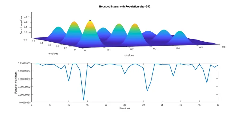
View 1

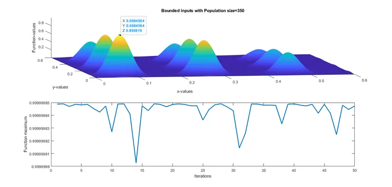
View 2

ERRORS FACED WHILE PROGRAMMING:

Error 1: Not saving the function file and the main program file in the same directory or folder.

Output due to the mistake:

Correction made: Saved the function file in the same folder as the main program file.

Error 2: Naming the program file as ‘ga.m’.

Output due to the mistake:

Correction made: Saved the main program file with some other name.

CONCLUSION:

The ‘ga’ solver/function in MATLAB is a powerful tool that can be used to give an optimized result/minima of a function which depends on 1 or more independent parameters. Via this project, we have seen how the ‘ga’ solver, which uses the fundamentals of genetic algorithm (based on theory of Natural Evolution) gave a possible set of solutions for the function and after some modifications in the inputs and applying it in the alternate syntaxes of the ‘ga’ solver, we could get an output that we are happy with.
The ‘ga’ solver is powerful tool in MATLAB which can be used to find the optimized solutions of many complex functions which may depend on many independent parameters. Thus this tool may prove to be useful in optimization of many complex engineering problems.

REFERENCES:

Genetic Algorithm Implementation using MATLAB Programming

Ship work like this
in your own course.

Talk to a career counsellor

Ship work like thisin your own course.

Talk to a career counsellor

Ship work like this
in your own course.