Rankine Cycle Simulator using MATLAB Programming

AIM:

• To calculate the thermodynamic properties at the important state points of a Rankine Cycle using the XSteam function. The inputs of the user are taken for initial thermodynamic values which will facilitate further calculations.
• To plot the corresponding T-s and h-s plots based on the calculated values and user inputs along with the Saturated Vapour Line and Saturated Liquid Line.
• To also calculate the Net Work Output and Back Work Ratio of the Rankine Cycle based on the values of the thermodynamic properties at the important state points.

GOVERNING EQUATIONS & RELEVANT THEORY:

• Rankine Cycle is a vapour power thermodynamic cycle. It means that in the cycle, the working fluid is alternately vaporized and condensed throughout the cycle. Working fluid is not in a single state through every part of the cycle.
• Rankine cycle is a closed cycle as the working fluid returns to initial state at the end of the cycle and re-circulated.
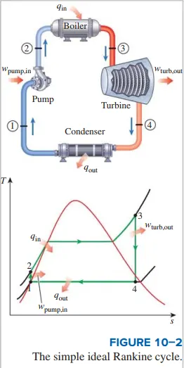
• An ideal Rankine Cycle consists of the 4 processes:
  • Process 1-2: Isentropic compression of working fluid in Pump at liquid state.
  • Process 2-3: Isobaric Heat addition to the working fluid in boiler changing its state from liquid to vapour.
  • Process 3-4: Isentropic expansion of working fluid in Turbine at vapour state.
  • Process 4-1: Isobaric Heat Rejection of working fluid in condenser bringing the working fluid back to saturated liquid state.

• Assumptions made for this project:
  • The Rankine Cycle is ideal(no internal irreversibilities in the cycle)
  • In an ideal Rankine Cycle, the working fluid enters the pump at saturated liquid state.
  • In an ideal Rankine Cycle, the working fluid enters the turbine at superheated vapour state.
  • In an ideal Rankine cycle, usually the working fluid enters the condenser inlet at saturated liquid-vapour state of high quality.
  • For this project, the state point 1(starting point of the cycle) is taken as the inlet of the turbine where the working fluid enters in a superheated vapour state.
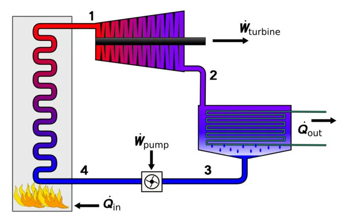
  • Therefore for this project sequence of processes for Rankine cycle is as follows:
  • Process 1-2: Isentropic Expansion of working fluid in Turbine at vapour state. (s₂=s₁)
  • Process 2-3: Isobaric Heat Rejection from working fluid in Condenser bring the working fluid to saturated liquid state. (P2=P3)
  • Process 3-4: Isentropic compression of working fluid in Pump at liquid state. (s₄=s₃)
  • Process 4-1: Isobaric Heat addition to the working fluid in boiler changing its state from liquid to vapour. (P4=P1)
  • For this project, the working fluid is water/steam because the XSteam function calculates all parameters for H2O.
  • The critical temperature of water is taken as: 373.95 °C

• The states of the working fluid(H₂O) at the state points are:
  • State point 1: Superheated Vapour State
  • State point 2: Saturated Liquid-Vapour mixture/Saturated Vapour/Superheated Vapour.
  • State Point 3: Saturated Liquid State.
  • State Point 4: Sub-cooled Liquid State.

• The individual processes in the Rankine cycle (Expansion, Compression, Heat Rejection, Heat Addition) are steady flow processes and take place in steady flow devices (Turbine, Compressor, Boiler, Condenser).
• Therefore to calculate the heat and work exchanges in each of these devices, we need to apply the Steady Flow Energy Equations(S.F.E.E.):
• After applying the S.F.E.E., we get the following equations:
  • w_out,Turbine = h₁ - h₂
  • w_in,Pump = h₄ – h_3­
  • q_in,Boiler = h₁ – h₄
  • q_{out,Condenser} = h₂ – h₃

where

1 -> Turbine inlet/Boiler outlet

2 -> Condenser inlet/Turbine outlet

3 -> Pump inlet/Condenser outlet

4 -> Boiler inlet/Pump outlet

h₁ -> specific enthalpy at state point 1

h₂ -> specific enthalpy at state point 2

h₃ -> specific enthalpy at state point 3

h₄ -> specific enthalpy at state point 4

P₁ -> Pressure at point 1

P₂ -> Pressure at point 2

P₃ -> Pressure at point 3

P₄ -> Pressure at point 4

s₁ -> Entropy at point 1

s₂ -> Entropy at point 2

s₃ -> Entropy at point 3

s₄ -> Entropy at point 4

w_out,Turbine -> work output by the turbine per unit mass

w_in,Pump -> work input to the pump per unit mass

q_{out,Condenser} -> heat rejected by system per unit mass

q_in,Boiler -> heat added to the system per unit mass

• w_net,out= w_out,Turbine - w_in,Pump = h₁ - h₂ - h₄ + h₃
• q_net,in = q_boiler,in - q_{condenser,out} = h₁ - h₄ - h₂ + h₃

where

w_net,out = Net work output per cycle

q_net,in = Net heat input per cycle

From the above 2 equations we can conclude that w_net,out = q_net,in which always holds true for a closed thermodynamic cycle.

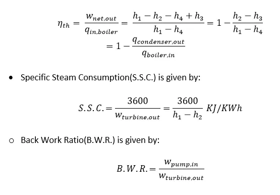
The thermal efficiency of the cycle is given by the following formula:

BODY OF THE CONTENT:

• Programming Language used: MATLAB
• I have been provided with a function file named XSteam.m which provides steam and water properties from 0 - 1000 bar and from 0 - 2000 °C according to the standard IAPWS IF-97.
• Using this XSteam.m function, I will calculate the various thermodynamic properties at the state points of the Rankine Cycle.
• The inputs for Turbine Inlet Temperature and Pressure along with the Condenser Inlet Pressure will be provided by the user.
• This initial values will pave the way for calculation of the other thermodynamic properties using the XSteam function.
• Attached below is the MATLAB code:

clear
close all
clc

disp('                                   RANKINE CYCLE SIMULATOR')
fprintf("n")
disp('1-2 is isentropic expansion in the turbine.')
disp('2-3 is isobaric heat rejection by the condenser.')
disp('3-4 is isentropic compression in the pump.')
disp('4-1 is isobaric heat addition by the boiler.')

%Getting the values of the thermodynamic properties at the state points either by user input or calling the XSteam function
for i=1:4
    
    if(i==1)
        %Getting the values of Pressure at all 4 state points and
        %Temperature at state point 1:
        P(i)=input('nEnter the Pressure at the Turbine inlet (in bar): ');
        T(i)=input('Enter the Temperature at Turbine inlet (in °C): ');
        P(i+1)=input('Enter the Pressure at the Condenser (in bar): ');
        P(i+3)=P(i);
        P(i+2)=P(i+1);
    end
    
    %Getting the Saturation Temperature and the specific entropy and
    %specific enthalpy for both saturated liquid and saturated vapour phase
    %corresponding to the Pressure values obtained:
    T_Sat(i)=XSteam('Tsat_p',P(i));
    h_Slp(i)=XSteam('hL_p',P(i));
    h_Svp(i)=XSteam('hV_p',P(i));
    s_Slp(i)=XSteam('sL_p',P(i));
    s_Svp(i)=XSteam('sV_p',P(i));
    
    
    %Obtaining the Temperature and Specific Entropy values:
    if (i==1) || (i==3)
        
        if(i==3)
            T(i)=T_Sat(i);
            s(i)=s_Slp(i);
        else
            s(i)=XSteam('s_pT',P(i),T(i));
        end
        s(i+1)=s(i);
        
    end
    
    if (i==2) || (i==4)   
        
        T(i)=XSteam('T_ps',P(i),s(i));
    end
    
    %Obtaining the specific enthalpy values corresponding to the Pressure and specific entropy values obtained: 
    h(i)=XSteam('h_ps',P(i),s(i));
    
    %Obtaining the dryness fraction values for all the 4 state points:
    if (T(i)==T_Sat(i))
        x(i)=(s(i)-s_Slp(i))/(s_Svp(i)-s_Slp(i));
    else
        x(i)="Not Applicable";
    end
   
end

%Conditions that won't fulfill criteria for Rankine Cycle:
if T(1)~=max(T) || s(1)<=s_Svp(1) || s(4)>=s_Slp(4) || P(1)<=P(2)
    fprintf("nThe inputs do not fulfill the basic criteria for an Ideal Rankine cycle")
    return
end

%Calculation of various parameters: 
W_TurbOut=h(1)-h(2);
W_PumpIn=h(4)-h(3);
q_BoilIn=h(1)-h(4);
q_CondOut=h(2)-h(3);

W_netOut=W_TurbOut-W_PumpIn;
q_netIn=q_BoilIn-q_CondOut;

N_therm=W_netOut/q_BoilIn;

BWR=W_PumpIn/W_TurbOut;

SSC=3600/(h(1)-h(2));

%Displaying the obtained Thermodynamic property values at all 4 state
%points and also displaying the calculated values of the parameters:
fprintf("nn                              RESULTS")
for i=1:4
    fprintf("nnAt State Point %d:",i)
    fprintf("nPressure at point %d (P%d) is : %.2f bar",i,i,P(i))
    fprintf("nTemperature at point %d (T%d) is : %.2f °C",i,i,T(i))
    fprintf("nSpecific Enthalpy at point %d (h%d) is : %.2f KJ/kg",i,i,h(i))
    fprintf("nSpecific Entropy at point %d (s%d) is : %.2f KJ/kgK",i,i,s(i))
    
    if x(i)~=("Not Applicable")
        fprintf("nDryness Fraction at point %d (x%d) is : %.2f",i,i,x(i))
    end
end

fprintf("nnWork output by the turbine per cycle (Wt) is : %.2f KJ/kg",W_TurbOut)
fprintf("nWork input to the pump per cycle (Wp) is : %.2f KJ/kg",W_PumpIn)
fprintf("nNet work output by the system per cycle (Wnet) is : %.2f KJ/kg",W_netOut)
fprintf("nThermal efficiency of the cycle (NTherm) is : %.2f",N_therm*100)
disp(' %')
fprintf("Specific steam consumption per cycle (S.S.C.) is : %.2f KJ/KWh",SSC)
fprintf("nBack work Ratio of the cycle (B.W.R.) is : %.4f",BWR)
    

%Plotting the T-s diagram and h-s curve using the obtained thermodynamic
%property values of the 4 state points:
for i=1:4
    if(i==4)  
        T(i+1)=T(i-3);
        P(i+1)=P(i-3);
        s(i+1)=s(i-3);
        T_Sat(i+1)=T_Sat(i-3);
        s_Slp(i+1)=s_Slp(i-3);
        s_Svp(i+1)=s_Svp(i-3);
        h(i+1)=h(i-3);
        h_Slp(i+1)=h_Slp(i-3);
        h_Svp(i+1)=h_Svp(i-3);
    end
    
    if (P(i)==P(i+1))
        if(s(i)>s(i+1))
            if (s(i)>=s_Svp(i) && s(i+1)>s_Slp(i+1))
                TRangeH2L1=linspace(T(i),T(i+1),5000);
                for k=1:length(TRangeH2L1)
                    sRangeH2L1(k)=XSteam('s_pT',P(i),TRangeH2L1(k));
                end
                figure(1)
                plot([s(i) sRangeH2L1 s_Svp(i) s(i+1)],[T(i) TRangeH2L1 T_Sat(i) T(i+1)],'Linewidth',2)
                hold on
            elseif (s(i)>=s_Svp(i) && s(i+1)<=s_Slp(i+1))
                TRangeH2L1=linspace(T(i),T_Sat(i),5000);
                TRangeH2L2=linspace(T_Sat(i),T(i+1),5000);
                for k=1:length(TRangeH2L1)
                    sRangeH2L1(k)=XSteam('s_pT',P(i),TRangeH2L1(k));
                end
                for m=1:length(TRangeH2L2)
                    sRangeH2L2(m)=XSteam('s_pT',P(i),TRangeH2L2(m));
                end
                figure(1)
                plot([s(i) sRangeH2L1 s_Svp(i) s_Slp(i+1) sRangeH2L2 s(i+1)],[T(i) TRangeH2L1 T_Sat(i) T_Sat(i+1) TRangeH2L2 T(i+1)],'Linewidth',2)
                hold on
            elseif (s(i)<s_Svp(i) && s(i+1)>s_Slp(i+1))
                figure(1)
                plot([s(i) s(i+1)],[T(i) T(i+1)],'Linewidth',1)
                hold on
            elseif (s(i)<s_Svp(i) && s(i+1)<=s_Slp(i+1))
                TRangeH2L2=linspace(T_Sat(i),T(i+1),5000);
                for m=1:length(TRangeH2L2)
                    sRangeH2L2(m)=XSteam('s_pT',P(i),TRangeH2L2(m));
                end
                figure(1)
                plot([s(i) s_Slp(i+1) sRangeH2L2 s(i+1)],[T(i) T_Sat(i+1) TRangeH2L2 T(i+1)],'Linewidth',2)
                hold on
            end
            
        elseif(s(i)<s(i+1))
            if (s(i)<=s_Slp(i) && s(i+1)<s_Svp(i+1))
                TRangeL2H1=linspace(T(i),T(i+1),5000);
                for n=1:length(TRangeL2H1)
                    sRangeL2H1(n)=XSteam('s_pT',P(i),TRangeL2H1(n));
                end
                figure(1)
                plot([s(i) sRangeL2H1 s_Slp(i) s(i+1)],[T(i) TRangeL2H1 T_Sat(i) T(i+1)],'Linewidth',2)
                hold on
            elseif (s(i)<=s_Slp(i) && s(i+1)>=s_Svp(i+1))
                TRangeL2H1=linspace(T(i),T_Sat(i),5000);
                TRangeL2H2=linspace(T_Sat(i),T(i+1),5000);
                for n=1:length(TRangeL2H1)
                    sRangeL2H1(n)=XSteam('s_pT',P(i),TRangeL2H1(n));
                end
                for p=1:length(TRangeL2H2)
                    sRangeL2H2(p)=XSteam('s_pT',P(i),TRangeL2H2(p));
                end
                figure(1)
                plot([s(i) sRangeL2H1 s_Slp(i) s_Svp(i+1) sRangeL2H2 s(i+1)],[T(i) TRangeL2H1 T_Sat(i) T_Sat(i+1) TRangeL2H2 T(i+1)],'Linewidth',2)
                hold on
            elseif (s(i)>s_Slp(i) && s(i+1)<s_Svp(i+1))
                figure(1)
                plot([s(i) s(i+1)],[T(i) T(i+1)],'Linewidth',2)
                hold on
            elseif (s(i)>s_Slp(i) && s(i+1)>=s_Svp(i+1))
                TRangeL2H2=linspace(T_Sat(i),T(i+1),5000);
                for p=1:length(TRangeL2H2)
                    sRangeL2H2(p)=XSteam('s_pT',P(i),TRangeL2H2(p));
                end
                figure(1)
                plot([s(i) s_Svp(i+1) sRangeL2H2 s(i+1)],[T(i) T_Sat(i+1) TRangeL2H2 T(i+1)],'Linewidth',2)
                hold on
            end
        end
    elseif (s(i)==s(i+1))
        figure(1)
        plot([s(i) s(i+1)],[T(i) T(i+1)],'Linewidth',2)
        hold on
    end
    
    figure(2)
    plot([s(i) s(i+1)],[h(i) h(i+1)],'Linewidth',2)
    hold on

end


%Obtaining the range of values of Saturation Temperature values for plotting the Saturated Liquid Line and the Saturated Vapour line: 
T_SatRange=linspace(0,373.95,1000);

%Obtaining the range of Saturation Pressure,Specific enthalpy and specific
%entropy at Saturated Liquid Phase and Saturated Vapour Phase corresponding
%to the obtained Saturation Temperature values:
for j=1:length(T_SatRange)
    P_SatRange(j)=XSteam('psat_T',T_SatRange(j));
    h_SlpRange(j)=XSteam('hL_p',P_SatRange(j));
    h_SvpRange(j)=XSteam('hV_p',P_SatRange(j));
    s_SlpRange(j)=XSteam('sL_p',P_SatRange(j));
    s_SvpRange(j)=XSteam('sV_p',P_SatRange(j));
    
        
    if (s_SlpRange(j)==s_SvpRange(j))
        Pcr=P_SatRange(j);
        Tcr=T_SatRange(j);
    end
end
    
%Plotting the [Saturation Temperature-Specific Entropy at Saturated Liquid Phase] diagram and [Saturation Temperature-Specific Entropy at Saturated Vapour Phase] on the obtained T-s curve:    
figure(1)
plot(s_SlpRange,T_SatRange,'Linewidth',1,'color','g','linestyle','--')
hold on
plot(s_SvpRange,T_SatRange,'Linewidth',1,'color','g','linestyle','--')
xlabel('Specific Entropy(KJ/kgK)')
ylabel('Temperature(°C)')
title('Temperature-Specific Entropy(T-s) Curve of the Rankine Cycle')
legend('Turbine','Condenser','Pump','Boiler')
grid on
hold off

%Plotting the [Specific Enthalpy at Saturated Liquid Phase-Specific Entropy at Saturated Liquid Phase] diagram and [Specific Enthalpy at Saturated Vapour Phase-Specific Entropy at Saturated Vapour Phase] on the obtained h-s curve:
figure(2)
plot(s_SlpRange,h_SlpRange,'Linewidth',1,'color','g','linestyle','--')
hold on
plot(s_SvpRange,h_SvpRange,'Linewidth',1,'color','g','linestyle','--')
xlabel('Specific Entropy(KJ/kgK)')
ylabel('Specific Enthalpy(KJ/kg)')
title('Specific Enthalpy-Specific Entropy(h-s) Curve of the Rankine Cycle')
grid on
hold off

• As per the question the following should be the format for the output:

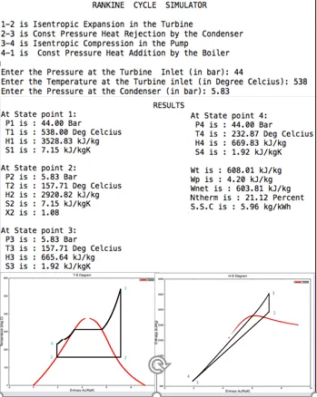
• Using the commands ‘disp’ and ‘fprintf’, I display the text ‘RANKINE CYCLE SIMULATOR’ and the next four lines describing the processes of the Rankine cycle on the command window.
• Next, I use the ‘input’ command which displays the question on the command window asking for an input and the next step of the program gets executed after the user gives an input.
• Using the input command, the program asks the user to specify the values of the Temperature & Pressure of the Turbine inlet and the Pressure of the condenser inlet.
• The next step involves finding various thermodynamic properties at the state points of the Rankine cycle. The values of these properties will be required for plotting the T-s diagram, h-s diagram and calculating various other parameters asked in the question.
• For finding out the values of the thermodynamic properties at the state points, the user needs to call the XSteam function.
• The XSteam function needs some suitable input arguments for calculation of the required thermodynamic properties.
• For calculation of the required thermodynamic property, what input argument needs to be specified for the calculation has been specified in the XSteam function definition along with comments describing it.
• I have used a ‘for’ loop for calculating the thermodynamic properties at all the state points.
• There are 4 state points where the thermodynamic parameters need to be calculated/input. Hence I have initialised the loop counter variable ‘i’ from 1 to 4, which indicates that the content within the ‘for’ loop will run 4 times.
• For the content inside the ‘for’ loop, an n^th loop run means that all the thermodynamic properties will be calculated/input for the n^th state point. Example: For the 2^nd loop run, the thermodynamic parameters for 2^nd state point will be calculated. This gets executed using the if/else statements inside the ‘for’ loop.
• However there are some thermodynamic properties which remain same in 2 state points like Entropy and Pressure. For example, in the expansion process of steam in the turbine is isentropic in nature i.e. the entropy remains constant throughout the process. Therefore s₁=s₂. Hence in the first loop run itself, I have assigned the entropy at state point 2 using equal to the entropy at state point 1.The entropy at state point 1 gets calculated using the XSteam function during the 1^st loop run itself.
• Similarly in this way the pressure values also get calculated. The Pressure values at inlet of Turbine and inlet of Condenser are user defined. The Pressure values at inlet of Pump and inlet of Boiler automatically gets assigned.
• Now for each loop run, the thermodynamic parameters like Saturation Temperature, Temperature, Specific Entropy, Specific Enthalpy ,Specific Entropy at Saturated Liquid Point for a particular pressure, Specific Entropy at Saturated Vapour point, Specific Enthalpy at Saturated Liquid point, Specific Enthalpy at Saturated Vapour point, Dryness fraction gets calculated.
• Now there are some basic criteria that need to be met for a thermodynamic cycle to be an ideal Rankine cycle:
  • The temperature at inlet of turbine/outlet of Boiler should be the maximum temperature in the entire cycle.
  • The specific entropy at inlet of the turbine should be greater than the specific entropy of the working fluid at saturated vapour state ‘for the same pressure’.
  • Similarly, the specific entropy at inlet of the boiler should be lesser than the specific entropy of the working fluid at saturated liquid state ‘for the same pressure’.
  • The pressure at turbine inlet should be greater than the pressure at condenser inlet (Needs to be kept in mind specifically for users who are giving the inputs).
  • The Pressure at Boiler inlet should be greater than the pressure at Pump inlet.
• If the above conditions are not met, I have written a code using ‘if’ statement and ‘return’ command to display a message in the command window saying that the user inputs don’t fulfil the basic criteria for a Rankine cycle and the instructing the program to stop executing the code any further.
• The next step involves calculation of parameters as mentioned in the question and displaying the values against the parameter name on the command window.
• Calculation of parameters: work output from turbine per cycle, work input to the pump per cycle, net-work output by the system per cycle, thermal efficiency of the cycle, Specific Steam Consumption per cycle and Back-Work Ratio of the cycle are calculated by defining variables according to the formulae discussed in ‘GOVERNING EQUATIONS & RELEVANT THEORY’ section.
• Displaying the parameters on the command window is done by using the commands ‘fprintf’ and ‘disp’. Format specifiers have also been used for displaying the output in a particular fomat.
• The next step involves plotting the T-s and h-s diagram. For plotting, I have again used the ‘for’ loop.
• Since I need to plot a closed curve, therefore I have initialised all thermodynamic parameters of the state point 1 to another additional state point 5.
• 

• There are regions along the Rankine cycle curve where the curve between the plots is not a straight line. This regions include the T-s co-ordinates for a constant pressure (isobaric) process outside the wet region (superheated steam region and sub-cooled liquid region).
• The temperature values in these region are obtained by the linspace command and the corresponding specific entropy values are obtained by calling the XSteam function inside a ‘for loop’ which gives a specific entropic value for all the temperature values.
• The plots between 2 state points which lie within such regions are obtained by joining all obtained temperature and specific entropy values within this state points.
• On execution of all the contents within the ‘for’ loop, the T-s and h-s curves are obtained.
• The next step involves plotting the saturated Liquid line and the saturated vapour line in the T-s curve and h-s curve.
• For plotting these lines, we need the Saturation Temperature values, specific entropy value at saturated liquid line and specific entropy value at saturated vapour line for plotting on the T-s plot. Similarly for plotting on h-s plot, we need the Saturation Temperature values, specific enthalpy value at saturated liquid line and specific enthalpy values at saturated vapour line. Against a Saturated Temperature value, we will get a specific entropy value at saturated liquid line and specific entropy value at saturated vapour line. Similarly we will also get a specific enthalpy value at saturated liquid line and specific enthalpy value at saturated vapour line against a particular Saturated Temperature value.
• For obtaining the values of saturated temperature I have used the linspace command to return 1000 equally spaced values from 0 °C(least temperature for water in liquid phase) to 373.95 °C(critical temperature of water).
• On obtaining the values of saturated temperature, the next step is to calculate the saturated pressure values (corresponding to saturated temperature values) and then finding out the specific entropy and specific enthalpy at saturated liquid phase and saturated gaseous phase using the XSteam function which will take the saturated pressure values as input argument.
• After finding out the values these plots of specific entropy at saturated liquid and saturated gaseous phase against the saturated temperature values are added to the T-s graph using commands like plot, hold on, xlabel, ylabel, title, legend, grid on, hold on, hold off.
• Similarly the plots of specific enthalpy at saturated liquid and saturated gaseous phase against the saturated temperature are added to the h-s graph using commands like plot, hold on, xlabel, ylabel, title, legend, grid on, hold on, hold off.

RESULTS:

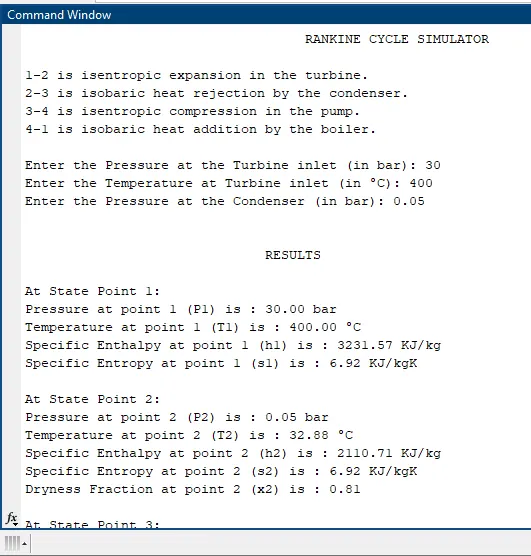
• On running the code, on the command window, the processes of the Rankine cycle were displayed and I was asked to enter the Turbine inlet Temperature and Pressure and also the Condenser inlet pressure.

Click on the link to see the execution of my code: https://drive.google.com/file/d/1fKXy2AU-yx-fgL4l1dmKmUmlPlAXGIjJ/view?usp=sharing

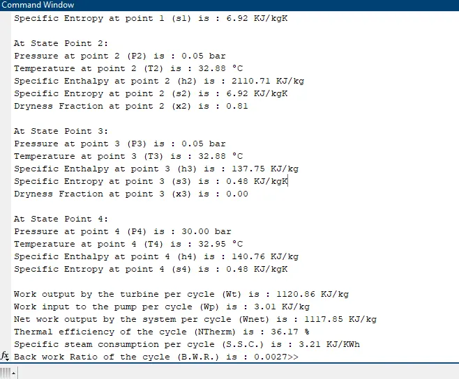
• On entering the input values as follows:

Enter the Pressure at the Turbine inlet (in bar): 30

Enter the Temperature at Turbine inlet (in °C): 400

Enter the Pressure at the Condenser (in bar): 0.05

T-s and h-s plots for the Rankine cycle corresponding to the user inputs were obtained.

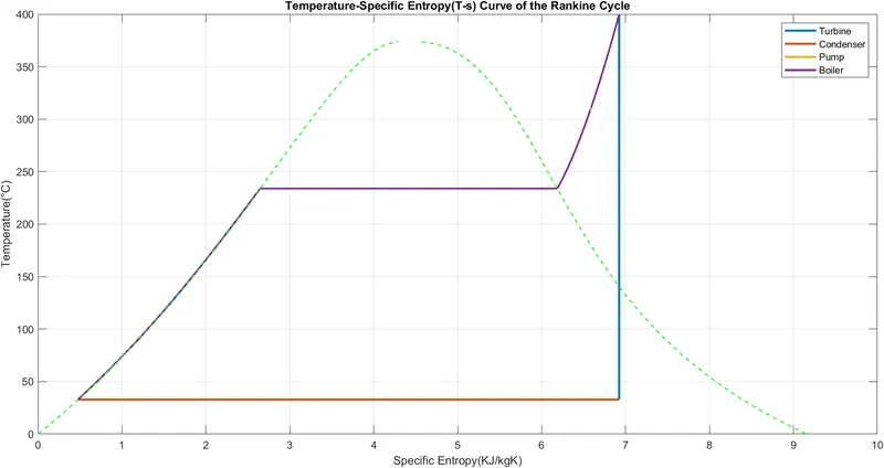
T-s plot (Note that Pump work not visible)

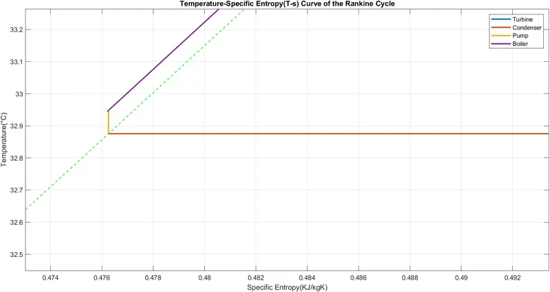
T-s diagram where the pump work (Yellow curve) has been emphasised which was other not visible

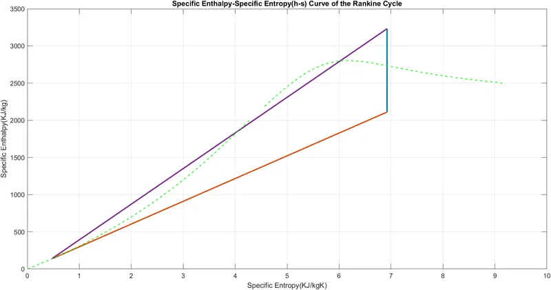
h-s plot (Again note that Process 3-4(const. entropy process) not visible(Yellow line))

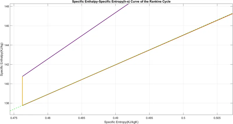
h-s plot where process 3-4(yellow line) which is a const. entropy process has been emphasized

• Also, the thermodynamic property values at 4 state points were displayed on the command window along with parameters (Thermal Efficiency, Back-Work Ratio, etc) as asked in the question.

1st Screenshot

2nd Screenshot

ERRORS MADE WHILE PROGRAMMING:

• Lots and lots of errors have been made by me while programming. Some of those errors were identified by MATLAB software during compilation of the code and error messages were generated in the command window. Those errors were rectified. Other errors made were correct as per the MATLAB syntax but the output generated by the code were different from expected results. These errors were identified in due time and the outputs generated after rectification were similar to the expected results.

CONCLUSIONS:

• MATLAB as a programming language and software can be used for diverse range of applications and operations catering to most engineering problems.
• As evident from the project, MATLAB can be used to calculate various engineering parameters by accessing the data of a function file and also plot the curve using the values of parameters obtained.
• It can also display all the values of the parameters on a separate window(command window).

REFERENCES:

• Thermodynamics: An Engineering Approach, Ninth Edition by Yunus A. Cengel, Michael A. Boles & Mehmet Kanoglu.
• https://www.sciencedirect.com/topics/engineering/back-work-ratio
• https://www.thermosolver.com/saturated
• http://www.expertsmind.com/topic/vapor-power-cycles/specific-steam-consumption-ssc-97681.aspx