P-V Diagram of an Otto Cycle & Thermal Efficiency Calculation of the Cycle using MATLAB Scripting

AIM:

1. To demonstrate the working of an Otto Cycle
2. To plot the P-V diagram of an Otto cycle and calculate the thermal efficiency of the cycle using MATLAB.

GOVERNING EQUATIONS & RELEVANT THEORY:

1. The Otto cycle is the ideal cycle for spark-ignition reciprocating engines.
2. In general, actual gas power cycles like Otto cycle are quite complex. To reduce the analysis to a manageable level, we utilize the following approximations with most being air standard assumptions:

• The working fluid is taken to be air, which continuously circulates in a closed loop and always behaves as an ideal gas.
• All the processes that make up the cycle are internally reversible.
• The combustion process is replaced by a heat-addition process from an external source.
• The exhaust process is replaced by a heat-rejection process that restores the working fluid to its initial state.
• Air has constant specific heats whose values are determined at room temperature (25^oC or 77^oF).
• All expansion and compression processes take place in a quasi-equilibrium manner.
• The system is considered to be closed i.e. there is no mass transfer between the system and surroundings but energy transfer can take place between the system and surroundings.
• The pipes connecting the various components of a system are well insulated, and heat transfer through them is negligible.
• Kinetic enery and potential energy changes are nergligible.

3. Before studying the Otto cycle process it is necessary to know about the parts in a reciprocating I.C. engine:

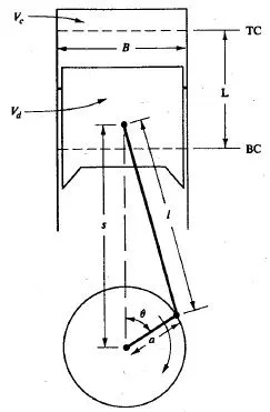
1. Cylinder: A cylindrical vessel or space in which the piston makes a reciprocating motion. The varying volume created in the cylinder during the operation of the engine is filled with the working fluid and subjected to different thermodynamic processes.
2. Piston: It is a cylindrical component fitted into the cylinder forming the moving boundary of the combustion system. It fits perfectly (snugly) into the cylinder providing a gas-tight space with the piston rings and the lubricant.
3. Combustion Chamber: The space enclosed in the upper part of the cylinder, by the cylinder head and the piston top during the combustion process is called combustion chamber. The combustion of fuel and the consequent release of thermal energy in results in the holding up of pressure in this part of the cylinder.
4. Connecting rod: It interconnects the piston and crankshaft and transmits the gas forces from the piston to the crankshaft.
5. Crankshaft: It converts the reciprocating motion of the piston into useful rotary motion of the output shaft.

4. Some important terminologies of a reciprocating engine(I.C. engine) on which this gas power cycles operate:
   1. Top dead centre (T.D.C.): The position of piston when it forms the smallest volume of the cylinder.
   2. Bottom dead centre (B.D.C.): The position of the cylinder when it forms the largest volume in the cylinder.
   3. Stroke (L): The distance between T.D.C. and B.D.C. is the largest distance that the piston can travel and it is called the stroke of the engine.
   4. Bore (d): The diameter of the piston is called bore.
   5. Intake valve: The air or air-fuel mixture is drawn into the cylinder through the intake valve.
   6. Exhaust valve: The combustion products are expelled from the cylinder through the exhaust valve.
   7. Clearance volume (V_c): The minimum volume formed in the cylinder when the piston is at T.D.C. is called the clearance volume.
   8. Displacement volume/Swept volume (V_s): The volume displaced by the piston as it moves between T.D.C. and B.D.C. is called displacement volume.
   9. Compression Ratio (c_r): The ratio of maximum volume (displacement volume + clearance volume) and minimum volume (clearance volume) is called the compression ratio of the cylinder.

Working of Ideal Otto cycle: The Otto cycle is the ideal cycle for spark ignition (S.I.) reciprocating engines. In most spark ignition engines, the piston executes four complete strokes (2 mechanical cycles) within the cylinder and the crankshaft completes 2 revolutions for each thermodynamic (Otto) cycle.

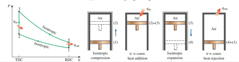
Ideal cycle in spark ignition engine (Otto cycle) and it’s P-v diagram.

Since for this project, the Otto cycle is ideal, I have assumed the cycle to be closed but the actual Otto cycle (in S.I. engines) is an open cycle.

Since the cycle is a closed cycle, therefore there is no mass exchange between the system and surroundings. Therefore for individual processes in the cycle like compression, expansion and combustion we can use the equation of 1^st law of Thermodynamics for closed systems.

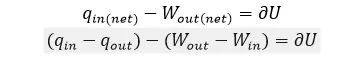
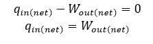
For the entire cycle, there is no change in internal energy. Therefore:

1. Process 1-2: This process represents isentropic (internally reversible and adiabatic) compression of the air when the piston moves from B.D.C. to T.D.C.

For process 1-2(Isentropic Compression):

q_in=q_out =0; W_out=0.

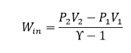
In actual S.I.(4 stroke) engine this process corresponds to the compression stroke, where the inlet and exhaust valve of the cylinder remains closed and during this process the crankshaft rotates from 180^o to 360⁰ thus revolving 180 degrees.

2. Process 2-3: During this process heat is supplied reversibly at constant volume while the piston remains at T.D.C.

For process 2-3(Constant volume heat addition):

q_out=0 ; W_in=W_out=0 as ΔV=0.

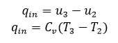
3. Process 3-4: This process represents isentropic expansion (internally reversible and adiabatic) expansion of air when the piston moves from T.D.C. to B.D.C.

For process 3-4: q_in=q_out=0 as process is isentropic ; W_in=0.

During this process, there is no heat exchange between system and surroundings. And there is a work output given by the system which is given by:

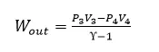
In actual S.I.(4 stroke) engine this process corresponds to that part of the power/combustion stroke, where after ignition of the working fluid causing an increase in pressure and temperature of the system pushes the piston down from T.D.C. to B.D.C. During this process the inlet and exhaust valve of the cylinder remains closed and during this process the crankshaft rotates from 0^o to 180⁰ thus revolving 180 degrees of the second mechanical cycle.

4. Process 4-1: During this process, heat is rejected reversibly by the system (air being the working fluid and the piston wall and the cylinder walls being the boundary) at constant volume while the piston remains at B.D.C.

For process 4-1(Constant volume heat rejection):

q_in=0 ; W_in=W_out=0 as ΔV=0.

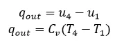
Now in order to plot the cycle and to understand how the graph is varying, we must know the relation between various state properties in the cycle and the values of these state properties.

The volume at T.D.C. (which corresponds to the maximum volume within which air (working fluid) operates) and the volume at B.D.C.(the minimum volume at which air(working fluid) operates) can be found out by relations where it depends on the some geometrical parameters of the reciprocating engine.

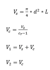where V_s = Swept volume V_c = Clearance volume

d = Cylinder Bore

L = Stroke

c_r = Compression Ratio

V₁ = Volume at T.D.C.

V₂ = Volume at B.D.C.

Process 1-2: Isentropic Compression.

Properties at state point 1: P₁, T₁ and V₁.

Properties at state point 2: P₂, T₂ and V₂.

Properties at state 1 are generally known as they are the initial conditions of the system. Therefore properties like P₁ and T₁ are known beforehand. Since 1->2 is an isentropic (adiabatic & internally reversible) process, therefore:

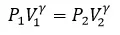
V₂ will be given as it corresponds to the clearance volume of the cylinder. From the above equation P₂ can be calculated as P₁, V₁, V₂ and ϒ are known.

After finding P₂ and knowing V₂, we can find out the value of T₂ using the relation:

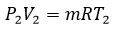
Where m is known and R=C_p-C_v is calculated beforehand.

Process 2-3: Isochoric Heat addition.

Properties at state point 2: P₂, V₂ and T_2.

Properties at state point 3: P₃, V₃ and T₃.

As of now, P₂, V₂ and T₂ are known. Since process 2->3 is an isochoric process, therefore we can say:

V₃=V₂ as the process is isochoric i.e. the volume remains constant during this process. Now considering that T₃ (which also happens to be the maximum temperature in the cycle) is known, P₃ (which is also the maximum pressure in the cycle) can be found out from the above relation.

Process 3-4: Isentropic expansion.

Properties at state point 3: P₃, V₃ and T₃.

Properties at state point 4: P₄, V₄ and T₄.

As of now, P₃, V₃ and T₃ are known. Since process 3->4 is an isentropic process, we can find out P₄. V₄ is known as it is equal to V₁ as we know in the process 3->4 the piston moves from T.D.C. (corresponds to V₂=V₃) to B.D.C. (corresponds to V₁=V₄).Therefore:

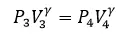
Using the above relation P₄ can be found out.

Thus, we now have the values of state properties required for plotting the P-V diagram of Otto cycle i.e. we have the values of P₁, P₂, P₃, P₄, V₁, V₂, V₃, V₄ .

The next step is to understand how the curve varies from one state point to another in a P-V diagram:

• Curve variation of process 2->3 and 4->1 will be a straight line as in this processes volume remains constant throughout the process.

For process 2->3, piston remains at B.D.C. and for process 4->1, the piston remains at T.D.C.

• Processes 1->2 and 3->4 are isentropic processes where P and V are related to each other in the following way:

Therefore, the variation of curve between the state points will depend on V,ϒ and the constant.

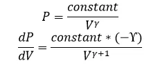
In real case scenario, the variation of the volume as the piston moves between T.D.C. and B.D.C. is given by the following relation (experimentally derived):

Where θ is the angle rotated by the crankshaft when the piston moves between T.D.C. and B.D.C. during an isentropic process.

where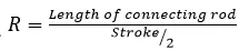

and c_r = Compression ratio.

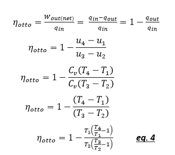
Now the thermal efficiency for the Otto cycle is given as follows:

As we know that for the entire cycle,

therefore:

For process 1->2 and 3->4 both are isentropic (internally reversible & adiabatic).Thus for both these processes:

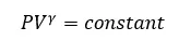eq. 1.

where = Specific heat ratio.

Since the working fluid is air which has been taken as an ideal gas, therefore we can say:

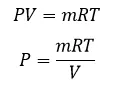
Substituting the value of P in eq. 1. we get:

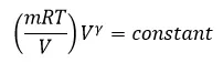
where m and R are constants. Therefore:

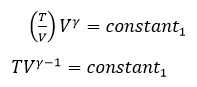
Therefore For process 1->2:

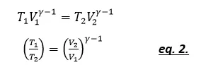
Again for process 3->4:

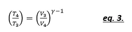
From previous relations we have seen V₂=V₃ and V₁=V₄.

Comparing eq. 2. and eq. 3 ,we can conclude:

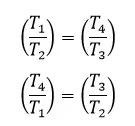
Using this relation in eq. 4( η_th(otto) expression), we get:

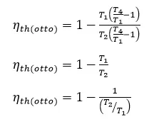
From eq. 2. We can say that:

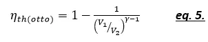
We also know that compression ratio (c_r) is given by:

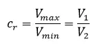
Substituting this value of V₁/V₂ in eq. 5 ,we get:

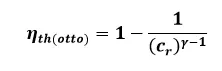
We will use the above expression to calculate the thermal efficiency of the Otto cycle.

BODY OF THE CONTENT:

1. Programming language used: MATLAB.
2. My MATLAB program for this project will consist of 2 separate files:
   1. One file is a function file which will take the input of the following geometrical parameters of the reciprocating engine from the main file:
      • Bore (value to be given during function call)
      • Stroke (value to be given during function call)
      • Connecting Rod length (value to be given during function call)
      • Compression ratio of the cylinder (value to be given during function call)
      • Angle at the start of the isentropic process. (value to be given during function call)
      • Angle at the end of the isentropic process. (value to be given during function call)

and define the following relations which will be instrumental in plotting and showcasing the curve variation for different processes in the ideal Otto cycle. The following relations will be defined where the terms in the relation are taken as arguments of the function:

• Relation which makes use of the above geometrical parameters where we can calculate the swept volume and clearance volume and hence calculate V₁ and V₂.
• Relation where we can calculate the value of V when the system is undergoing an isentropic process (i.e. we can calculate the volume using the relation and hence find out how the volume varies when the piston moves between T.D.C. and B.D.C. during an isentropic process).This relation will help in plotting the variation of curve for isentropic processes in a P-V diagram.

The function code is attached below:

function [V]=OttoCyclePistonKinematics(bore,stroke,con_rod,cr,start_crank,end_crank)   %(A function named OttoCyclePistonKnematics is declared that accepts inputs:bore,stroke,con_rod,cr,start_crank,end_crank and returns output of variable V)

%Inputs:
a=stroke/2;                 %(Intialised a variable 'a' that will take the value of variable stroke and divide it 2) 
R=con_rod/a;                %(Intialised a variable 'R' that will store the value of (con_rod/a))
v_s=pi/4*bore^2*stroke;     %(Initialised a variable 'v_s' that will store the value of (pi/4*bore^2*stroke))
v_c=v_s/(cr-1);             %(Initialised a variable 'v_c' that will store the value of (v_s/(cr-1))

theta=linspace(start_crank,end_crank,100);      %(Initialised an arrary 'theta' that will store 100 values equally distributed from 'start_crank' to 'end_crank')
term1=0.5*(cr-1);                               %(Initialised a variable 'term1' that will store the value of (0.5*(cr-1)))
term2=R+1-cosd(theta);                          %(Initialised a variable 'term2' that will store the value of (R+1-cosd(theta)))
term3=(R^2-sind(theta).^2).^0.5;                %(Initialised a variable 'term3' that will store the value of ([R^2-sind(theta).^2].^0.5))
V=(1+term1*(term2-term3)).*v_c;                %(Initialised a variable 'V' that will store the value of ((1+term1.*(term2-term3)).*v_c))


end                                     %(command to signal the end of content to be taken within the function)

1. The above code has been written in the Editor window of MATLAB.

• In MATLAB, anything written at a particular line starting with the special character '%' are comments for this programming language. The compiler skips anything that starts with '%' in a line while compiling and running the code.
• For the above case, I have used comments beside the code in each and every line to explain the functionality of that particular code.
• In order to show the calculation, plotting and hence variation of curves between [state point 1 and state point 2] and between [state point 3 and state point 4], the above function code is necessary to show the actual variation of volume of the system during an isentropic process.
• As evident from the function code the volume of the system during an isentropic process depends on the crank angle, bore, stroke, length of the connecting rod and compression ratio.
• The volume of the system in an isentropic process varies w.r.t. to crank angle and all the other parameters remain constant.
• The function returns the value of volume for every crank angle. Since the crank angle has been defined as an array of 100 values, therefore the variable ‘V’(corresponding to volume) has been defined in a way(using element wise operators) to return a value of volume for every value of ‘θ’(corresponding to crank angle).
• Hence, the variable ‘V’ will return a row vector of 100 values.

1. The main program code is attached below:

clear        %(clears the previous variables and their intialised values if any.)
close all    %(closes all the output windows of MATLAB if any.)
clc          %(clears all the syntax and code previously written if any.)


%Inputs:
gamma=1.4;      %(Initialised a variable with a value of 1.4)

%State variables Input:
p1=101325;              %(Intialised a variable 'p1' with a value of 101325)
t1=500;                 %(Initialised a variable 't1' with a value of 500)
t3=2000;                %(Initialised a variable 't3' with a value of 2000)

%Engine geometric parameters:
bore=0.05;              %(Initialised a variable 'bore' with a value of 0.05)
stroke=0.1;             %(Initialised a variable 'stroke' with a value of 0.1)
con_rod=0.15;           %(Initialised a variable 'con_rod' with a value of 0.15)
cr=3;                   %(Initialised a variable 'cr' with a value of 3)


%Calculating the swept volume and clearance volume:
v_swept=(pi/4)*bore^2*stroke;       %(Intialised a variable 'v_swept' that will store the value of (pi/4)*bore^2*stroke))
v_clearance=v_swept/(cr-1);         %(Intialised a variable 'v_clearance' that will store the value of (v_swept/(cr-1)))
v1=v_swept+v_clearance;             %(Intialised a variable 'v1' that will store the value of (v_swept+v_clearance))
v2=v_clearance;                     %(Intialised a variable 'v2' that will store the value of (v_clearance))

%State variables of state point 2:
%p2v2^gamma=p1v1^gamma -> Relation that connects pressure and volume of state point 1 and state point 2 
%p2=p1*(v1/v2)^gamma=p1*cr^gamma -> Extension of the above relation where (v1/v2) has been substituted by cr 

p2=p1*cr^gamma;                     %(Intialised a variable 'p2' that will store the value of (p1*cr^gamma))

%p1v1/t1=p2v2/t2|t2=p2*v2*t1/(p1*v1) -> Ideal gas relation as the working fluid in system is air(ideal gas)
t2=p2*v2*t1/(p1*v1);                %(Initialised a variable 't2' to store the value of (p2*v2*t1/(p1*v1)))

%Function call for isentropic compression:
V_compression=OttoCyclePistonKinematics(bore,stroke,con_rod,cr,180,360);      %(Command for calling the function named OttoCyclePistonKinematics providing the necessary arguments for the function to execute and storing the the output of the function in the variable 'V_compression')   
constant_c=p1*v1^gamma;                                                     %(Initialised a variable 'constant_c' to store the value of (p1*v1^gamma))
P_compression=constant_c./V_compression.^gamma;                             %(Intialised a variable P_compression to store the values of (constant_c./V_compression.^gamma))     

       
%State variables at point 3:
p3=p2*t3/t2;                        %(Initialised a variable 'p3' to store the value of (p2*t3/t2))
v3=v2;                              %(Initialised a variable 'v3' to store the value of (v2))       

%State variables at point 4:
v4=v1;                              %(Initialised a variable 'v4' to take the value assigned to variable 'v1')
%p3v3^gamma=p4v4^gamma|p4=p3(v3/v4)^gamma -> Relation that connects pressure and volume of state point 3 and state point 4 
p4=p3*(v3/v4)^gamma;                %(Intialised a variable 'p4' that will store the value of (p3*(v3/v4)^gamma))

%Function call for expansion:
constant_c1=p3*v3^gamma;                                                    %(Initialised a variable 'c1' to store the value of (p3*v3^gamma))
V_expansion=OttoCyclePistonKinematics(bore,stroke,con_rod,cr,0,180);      %(Command for calling the function named OttoCyclePistonKinematics providing the necessary arguments for the function to execute and storing the the output of the function in the variable 'V_expansion')
P_expansion=constant_c1./V_expansion.^gamma;                                %(Intialised a variable P_expansion to store the values of (constant_c./V_expansion.^gamma))

%Plotting the graph:
figure(1)                                                                   %(Command to create the 1st figure window)
hold on                                                                     %(Command to retain plots in the current axes so that new plots added to the axes do not delete existing plots)
plot(V_compression,P_compression,'Linewidth',3)                             %(Command to plot the co-ordinates of (V_compression,P_compression) on the figure window and the width of the plots will be 3 units)          
plot([V_compression(end) v3],[P_compression(end) p3],'Linewidth',3)         %(Command to plot the last co-ordinate of (V_compression,P_compression) and co-ordinate of (v3,p3) and join them by straight line and the width of this straight line will be 3 units)
plot(V_expansion,P_expansion,'Linewidth',3)                                 %(Command to plot the co-ordinates of (V_expansion,P_expansion) on the figure window and the width of the plots will be 3 units)
plot([V_expansion(end) v1],[P_expansion(end) p1],'Linewidth',3)             %(Command to plot the last co-ordinate of (V_expansion,P_expansion) and co-ordinate of (v1,p1) and join them by straight line and the width of this straight line will be 3 units)
hold off                                                                    %(Command to set the hold state to off so that new plots added to the axes clear existing plots and reset all axes properties)    
grid on

%Adding labels to the axes of the figure window:
xlabel('Volume(m^3)')                               %(Command to label the x-axis of the graph as Volume(m^3))
ylabel('Pressure(Pa)')                              %(Command to label the y-axis of the graph as Pressure(Pa))

%Adding title and legends to the the graph:
title('P-V diagram of an ideal Otto Cycle')       %(Command to add title to the graph as 'P-V diagram of an ideal Otto Cycle')
legend('Isentropic Compression','Isochoric Heat Addition','Isentropic Expansion','Isochoric Heat Rejection')        %(Command to add legends to the graph where each legend in the command are sequentially arranged as per the order in which plot commands have been declared in the program. Therefore each legend depicts it's cooreponding plot in the order)  )

%Calculating thermal efficiency of the cycle:
eta=1-(1/(cr)^(gamma-1));                                                   %(Initialised a variable 'eta' to store the value of (1-(1/(cr)^(gamma-1))))
disp(['The thermal efficiency of the cycle is: ',num2str(eta*100),' %']);   %(Command to diplay 'The thermal efficiency of the cycle is: (the value of (eta*100)%') 

1. The above code has been written in the Editor window of MATLAB.

1. In MATLAB, anything written at a particular line starting with the special character '%' are comments for this programming language. The compiler skips anything that starts with '%' in a line while compiling and running the code.
2. For the above case, I have used comments beside the code in each and every line to explain the functionality of that particular code.
3. In the above code, all the geometrical parameters required for calculating, plotting and representing the variation of system volume during an isentropic process have been initialised.
4. The initial state properties (pressure and volume) required for calculating, plotting and representing the individual processes of the cycle as well as the entire cycle have also been initialised first.
5. For my project, I have initialised the parameters with the following values:
   • Specific heat ratio (ϒ) of air=1.4

In code the value corresponds to variable ‘gamma’

• Pressure at state point 1(P_1­)=101325 Pa

In code the value corresponds to variable ‘p1’

• Temperature at state point 1(T₁)=500 K

In code the value corresponds to variable ‘t1’

• Temperature at state point 3(T₃)=2000 K

In code the value corresponds to variable ‘t3’

• The value of bore(d) of cylinder assumed=0.05 m

In code the value corresponds to variable ‘bore’

• The value of stroke(L) assumed=0.1 m

In code the value corresponds to variable ‘stroke’

• The value of connecting rod length assumed=0.15 m

In code the value corresponds to variable ‘con_rod’

• The value of compression ratio assumed(c_r)=3

In code the value corresponds to variable ‘cr’

From there on, the state properties for the P-V diagram are calculated using the ideal gas law for isentropic process and isochoric process and plotted.

• By default, using the plot command between two co-ordinate points, MATLAB joins these 2 co-ordinates using a straight line.
• Hence, it was necessary to declare a separate function file for isentropic process as in P-V diagram the process is not represented as a straight line.
• Using that separate function file OttoPistonCycleKinematics, we plotted 100 discrete points from the initial start point of isentropic process to the end point. Joining these 100 points together gives a fair and smooth representation of the isentropic process curve.
• After plotting the processes, we get to represent the variation of the curve for all individual processes of the ideal Otto cycle on a P-V diagram.
• At the last stage of the program, the thermal efficiency of the ideal Otto cycle is calculated wherein a variable is used to calculate the value of thermal efficiency using the required formula and the result is displayed on the Command Window of the MATLAB software.

RESULTS: On running the code, the following output comes:

1. The following plot is obtained:

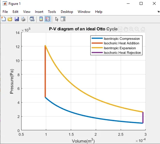
1. The output generated in command window:

ERRORS FACED WHILE PROGRAMMING:

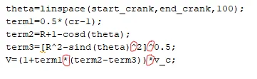
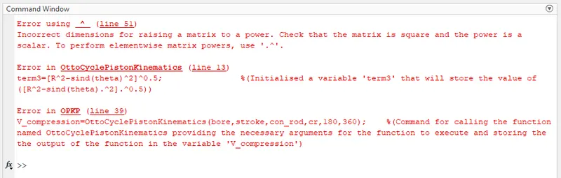
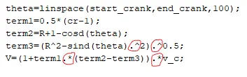
• Error 1: Forgetting use of element-wise operators at the required place whenever operations involving arrays/matrices come up.

In the function file I have declared the variable ‘theta’ as an array of 100 values. The compiler computes the value of ‘V’ using a very complex formula defined in the function which involves multiplication and exponentiation. In order to ensure that the necessary mathematical operation is done on every single value stored in ‘theta’ we need to apply element-wise operator wherever required. In short for such operations, dimensions of operands should be compatible for matrix operations.

Mistake made:

Output due to mistake:

Correction made: Using element wise operators instead of normal operators at the required positions. The syntax for element wise operator always starts with a ‘.’ followed by the operator as shown below:

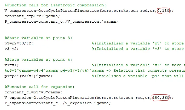
• Error 2: Putting wrong arguments/wrong order while calling function to compute volume array (V_compression,V_expansion).

While calling function to compute the values of volume for isentropic compression and isentropic expansion, I put the start_crank, end_crank values for function call of isentropic compression in wrong order.

The function has been defined to take arguments in a particular sequence only. While calling the function, it is necessary to put the arguments in the right sequence, otherwise an error may be generated while compiling or a wrong output may be generated.

For an ideal Otto cycle , the process of isentropic compression corresponds to the compression stroke in the S.I. engine and the crankshaft revolution starts at 180^o angle of crankshaft and ends at 360^o angle of crankshaft. Thus the crankshaft has revolved 180 degrees from 180^o position to 360^o position.

The process of isentropic expansion in the ideal Otto cycle corresponds to the power stroke in the S.I. engine and the crankshaft revolution (2^nd mechanical cycle) starts at 180^o angle of crankshaft and ends at 180^o angle of crankshaft. Thus the crankshaft has revolved 180 degrees from 0^o position to 180^o position.

Therefore for isentropic compression:

start_crank(corresponding to the angular position of crank at the start of process)=180

end_crank(corresponding to the angular position of crank at the end of process)=360 or 0

Therefore for isentropic expansion:

start_crank(corresponding to the angular position of crank at the start of process)=0 or 360

end_crank(corresponding to the angular position of crank at the end of process)=180

Mistake made: Interchanged the start_crank and end_crank values of Isentropic compression with the start_crank and end_crank values of Isentropic expansion. Or we can also say that I put the values for start_crank and end_crank in wrong order for both isentropic processes i.e. I put the end_crank value for start_crank palce and start_crank value in end_crank place for both isentropic processes. The start_crank value needs to be put first and then the end_crank value.

Output due to this mistake:

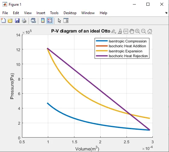
This output comes due to the fact that last values of the V_compression and V_expansion array calculated using the geometrical formula defined in the function does not match the value of v2(Clearance volume) and v4(Clearance volume+ swept volume) respectively.

Similarly the first values of the V_compression and V_expansion array calculated using the geometrical formula defined in the function does not match the value of v1(Clearance volume+ swept volume) and v3(clearance volume) respectively.

Correction made:

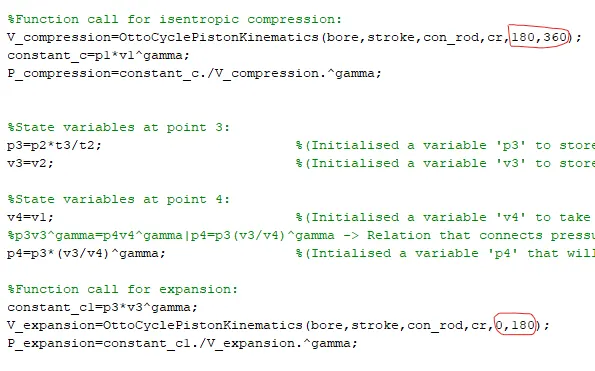
As seen from the correction, the right arguments for start_crank and end_crank for function OttoPistonCycleKinematics during the function call for Isentropic compression and isentropic expansion have been given and that too in the right sequence.