Motion of a Simple Pendulum Solution using MATLAB Programming
AIM:
- To write a program that solves the Ordinary Differential Equation representing the motion of a simple pendulum (with damping).
- To plot the variation of angular displacement and angular velocity (both obtained from solution of O.D.E.) w.r.t. time.
- To simulate the motion of the pendulum after obtaining the solution(s).
GOVERNING EQUATIONS & RELEVANT THEORY:
- Newton’s second law governs the motion of a simple pendulum.
- Using Newton’s 2nd law, we come at the equation of a simple pendulum which is a second order Ordinary Differential Equation (O.D.E.).
- This equation describes the position of the pendulum “bob” w.r.t. time.
- The equation is as follows:
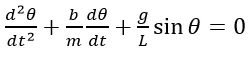
where g=acceleration due to gravity in m/s2
L= Length of pendulum (in m)
m=mass of bob (in kg)
b=damping coefficient.
θ=Angle made by the pendulum string w.r.t. the vertical axis.
t=time period of oscillation of pendulum.
- To solve an O.D.E. in MATLAB, we’ll need to use the ode45 function which is an in-built MATLAB function.
- ode45 function is only applicable for 1st order O.D.E.
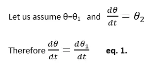
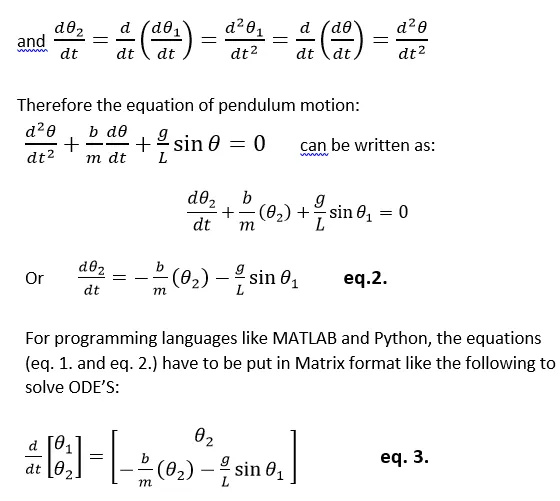
- Therefore in order to solve higher order O.D.E.(starting from 2nd order) using ode45, it is necessary to convert a higher order O.D.E. to a 1st order O.D.E.
This can be done in the following away:
BODY OF THE CONTENT:
- Programming language used: MATLAB.
- At first a function file is created in MATLAB that takes the following arguments:
- t (represents time)
- theta (represents θ which we have to find out)
- b (represents damping coefficient)
- g (represents acceleration due to gravity)
- m (represents mass of the bob)
- l (length of the string of pendulum)
Attached below is the function file:
function [dtheta_dt]=ode_func(t,theta,b,g,l,m)          %(A function named ode_func is declared that accepts inputs:t,theta,b,g,l,m and returns output whic gets initialised to array [dtheta_dt])

theta1=theta(1);                        %(Initialised a variable theta1 that will take the value of array 'theta' present at first index)
theta2=theta(2);                        %(Initialised a variable theta2 that will take the value of array 'theta' present at second index)
dtheta1_dt=theta2;                                  %(Intialised a variable 'dtheta1_dt' that will take the value of theta2)
dtheta2_dt=-(b/m)*theta2-(g/l)*sind(theta1);        %(Intialised a variable 'dtheta2_dt' that will store the value of (-(b/m)*theta2-(g/l)*sind(theta1)))
dtheta_dt=[dtheta1_dt;dtheta2_dt];                  %(Intialised a (2 X 1) matrix 'dtheta_dt' that will store the value of dtheta1_dt in the 1st row and dtheta2_dt in the 2nd row)
end %(command to signal the end of content to be taken within the function)- The above attached function basically takes the variables ‘t’, ‘theta’, ‘b’, ‘g’, ‘l’, ‘m’ and returns the value of the variable ‘dheta_dt’ as an output.
- In the function definition, I have written a code to create a matrix equation of the form θ’ = f(t) where θ’ is the variable matrix of order (2 X 1) and R.H.S. is a function of t (independent variable) also of order (2 X 1).
- The above function is necessary to implement the ode45 function for solving O.D.E.’s .
- Now in the main program, we will use the ode45 function to solve the ordinary differential equation in the matrix format as mentioned in eq. 3.
Attached below is the main program code:
clear               %(clears the previous variables and their intialised values if any.)
close all           %(closes all the output windows of MATLAB if any.)
clc                 %(clears all the syntax and code previously written if any.)

%Inputs:
b=0.05;             %(Initialised a variable 'b'(signifies damping coeffcient) with a value of 0.05)
g=9.81;             %(Initialised a variable 'g'(signifies acceleration due to gravity) with a value of 9.81)
l=1;                %(Initialised a variable 'l'(signifies length of the pendulum string) with a value of 1)
m=1;                %(Initialised a variable 'm'(signifies mass of the bob) with a value of 1)

%Initial conditions:
theta_0=[0;5];          %(Initialised a column matrix 'theta_0'(signifies intial values of angular displacement and angular velocity) of order (2 X 1)  with values of '0' at 1st row and '5' at 2nd row)

%Time points:
t_span=linspace(0,20,500);      %(Initialised a variable 't_span'(signifies the limits for time to be taken for solving the equation) with 500 equally spaced values starting from 0(lower limit) and ending at 20(upper limit))

%solve ODE:
[t,results]=ode45(@(t,theta) ode_func(t,theta,b,g,l,m),t_span,theta_0);     %(Implemented the ode45 function to solve the ODE and the output is in the form of a (500 X 3) matrix assigned to [t results])

ct=1;                                   %(Initialised a variable 'ct' with a value of 1)

%Plotting & adding legends:
figure(1)                               %(Command to create the 1st figure window)
plot(t,results(:,1),'Linewidth',2)      %(Command to plot the co-ordinates of (t,1st column of results matrix) on the figure window and the width of the plot will be 2 units)
hold on                                 %(Command to retain plots in the current axes so that new plots added to the axes do not delete existing plots)
plot(t,results(:,2),'Linewidth',2)      %(Command to plot the co-ordinates of (t,2nd column of results matrix) on the figure window and the width of the plot will be 2 units)
ylabel('Plot')                          %(Command to label the y-axis of the graph as 'Plot')
xlabel('Time')                          %(Command to label the x-axis of the graph as 'Time')
legend('Anglular displacement(degrees)','Angular Velocity(degress/second)');
for i=1:500                             %(Command to run the following contents inside this for loop 10 times)

    %Defining the co-ordintes of the pendulum cord:
    figure(2)                               %(Command to create the 2nd figure window)
    x0=0;                                   %(Initialised the x-co-ordinate of the extreme fixed end of the pendulum string to '0')
    y0=0;                                   %(Initialised the y-co-ordinate of the extreme fixed end of the pendulum string to '0')
    x1=-l*sind(results(i,1));               %(Initialised the x-co-ordinate of the free end of the pendulum srring to take the value (-l*sind(results(i,1)))
    y1=-l*cosd(results(i,1));               %(Initialised the y-co-ordinate of the free end of the pendulum srring to take the value (-l*cosd(results(i,1)))

    %Plotting for simulation:
    plot([x0 x1],[y0 y1],'Linewidth',3)     %(Command to plot a line between (x0,yo) and (x1,y1) and setting the width of the lines to 3 units)
    hold on                                 %(Command to retain plots in the current axes so that new plots added to the axes do not delete existing plots)
    plot(x1,y1,'o','MarkerFaceColor','red')     %(Command to put a marker(signifies bob of pendulum) at (x1,y1) and putting it's color as red)
    hold off                                %(Command to set the hold state to off so that new plots added to the axes clear existing plots and reset all axes properties)
    axis([-0.25 0.25 -1 0])               %(Setting the axis limits from -0.5 to 0.5 units in the x-axis and from -1.5 to 0.5 in the y-axis)

    title(['Simulation of pendulum motion at time =',num2str(t_span(i)),' seconds'])                    %(Adding a title on the top of the graph where time values are displayed for every corresponding position of pendulum cord)
    M(ct)=getframe(gcf);                    %(Command to capture images/frames of plots for every single unique position of pendulum cord and assigning them to a variable 'M')
    ct=ct+1;                                %(Incrementing the counter loop variable 'ct' by 1 every time the loop runs.)

end                                     %(Command signalling the end of the content to be taken for running the loop)

%Creating a video file which shows the simulations of frames captured:
movie(M)                %(movie(M) plays the movie frames in array M once)
videofile=VideoWriter('PendulumSimulation.avi','Uncompressed AVI');     %(Using a VideoWriter object to create a video file from the array M and assigning it to a variable named 'videofile')
open(videofile)                 %(Command to open a file assocoiated with 'videofile' for writing.)
writeVideo(videofile,M)         %(writeVideo command writes one or more movie frames typically returned by the getframe function)
close(videofile)                %(Command to close the video file assocoiated with 'videofile' to ensure that all data is written to the file.)
- In MATLAB, anything written at a particular line starting with the special character '%' are comments for this programming language. The compiler skips anything that starts with '%' in a line while compiling and running the code.
- For the above case, I have used comments beside the code in each and every line to explain the functionality of that particular code.
- In general, in order to solve partial/ordinary differential equations, where ‘θ’ is the dependent variable and ‘t’ is the independent variable, we solve ‘θ’ by integrating ‘dθ’ provided there are limits of integration.
- But for solving ordinary differential equations in MATLAB, we need to use a MATLAB ODE solver like ode45 which basically makes use of numerical methods to solve ordinary differential equations.
- Therefore rather than direct integration, ode45 will use a numeric solver to solve the equation. This is done by discretising the equation which involves:
- Converting O.D.E. into a linear equation.
- Solving this equation using a numerical method to find an approximate solution to the equation.
- The ode45 function takes 3 inputs:
- The function to be integrated.
- The Integration limits.
- The solution of the equation at an initial condition.
- In the above code, I have first defined the solution of the equation at an initial condition i.e. initially the value of θ1 and θ2 is defined as 0 and 5 respectively.
- Then the integration limits for the time (independent variable) has been defined as a row matrix of 500 equally spaced values with a lower limit value of 0 seconds and the upper limit value of 20 seconds.
- Therefore the initial solution of the equation is θ1=0(angular displacement) and θ2=5(angular velocity) at t=0 seconds(time).
- Then I have used the ODE solver ode45 which takes the input of the function(created as a separate function file where function name is ode_func) to be solved, the limits of time (t_span) for integration, and the initial value of the solution variables (theta1 and theta2) and the independent and dependent variable(t and theta).
- The output of the ode45 function is assigned to 2 variables ‘t’ and ‘results’ where the variable ‘t’ will correspond to the time matrix(named as t_span in the program) and will have all the 500 values of t_span in the form of column matrix.
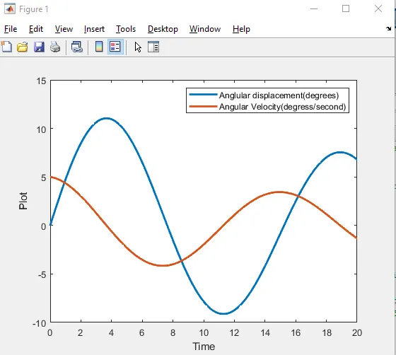
- The variable ‘results’ will contain the values of theta1 and theta2 of the function file in the form of a (500 X 2) matrix where the 1st column of 500 rows corresponds to the 500 solutions of θ1 (theta1 of ode_func function) where each value of θ1 corresponds to the time in the same row number of the column matrix ‘t’.
- Similarly, the 2nd column of the ‘results’ variable having 500 rows corresponds to 500 solutions of θ2 (theta2 of ode_func function) where each value of θ2 corresponds to the time in the same row number of the column matrix ‘t’.
- Thus we get the value of ‘θ1‘ and ‘θ2’(from the ‘results’ variable) for every corresponding value of ‘t’(corresponding to ‘t’ variable).
- θ1=θ as assumed in the ‘GOVERNING EQUATIONS & RELEVANT THEORY’ portion. This θ1=θ corresponds to angular displacement of the pendulum string/bob w.r.t. to the vertical axis. It’s unit is degrees.
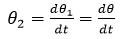 as assumed in the ‘GOVERNING EQUATIONS & RELEVANT THEORY’ portion. This θ2 corresponds to angular velocity of the pendulum bob while oscillating. It’s unit is degrees/second.
- Thus we have got the values of angular displacement and angular velocity for every value of time (taken 500 values from 0 seconds to 20 seconds).
- After getting the output, we plot values of θ1 and θ2 against it’s corresponding values of ‘t’ using the plot command.
- And in the end, I simulate the motion of the pendulum using the values of θ1 and time(t) using the ‘for’ loop. The loop runs for 500 times (corresponding to the no. of time values) and captures the co-ordinates of the pendulum string’s free end which is attached to the pendulum bob (which changes because θ1 changes as function of time) and the other end is fixed. For the sake of simplicity the pendulum string has been assumed to be a rigid link whose motion is dictated by the motion of the pendulum bob attached at it’s free end.
- After plotting the link we use the MATLAB functions like getframe, movie, VideoWriter, open, writeVideo and close to capture the frames of each distinct plot and use the frames to create a video/movie/simulation of the plots.
RESULTS:
- The following plot depicting the relationship between Angular displacement of the pendulum w.r.t. time(0-20 seconds) and the angular velocity of the pendulum w.r.t. time(0-20 seconds):
- The following animation depicting the simulation of the pendulum is obtained:
*Click on this link:* https://drive.google.com/file/d/1NonMtHwD1GgSPVWhE-IpB3kZARlde2iG/view?usp=sharing
ERRORS FACED WHILE PROGRAMMING:
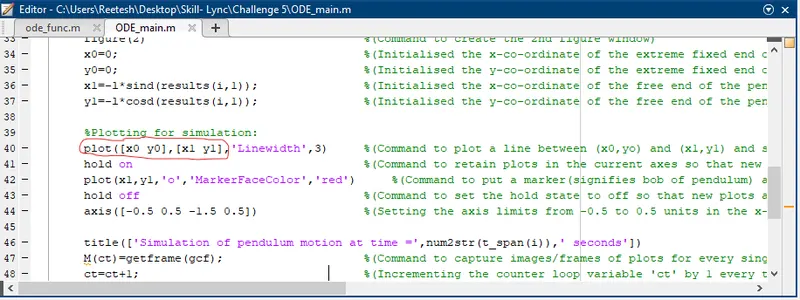
- Error 1: Wrong MATLAB syntax for plotting of graphs:
In general we identify a point in a graph by it’s x co-ordinate and y-co-ordinate and represent that point as (x, y) where x and y are the x co-ordinate and y-co-ordinate of that point respectively. Hence in order to join any two points in a graph, it’s representation using pen & paper is generally done by join (x0, y0) and (x1, y1). There is a huge chance that a MATLAB programmer will pass the syntax as:
plot ([x0,y0],[x1 y1])
to join these two points.
However this syntax in MATLAB is wrong as we need to write x- co-ordinates of both points first in square brackets and then write the y- co-ordinates of both the points in square brackets.
Mistake made:
Output due to this error:
*Click on the Link:*https://drive.google.com/file/d/1Z0OBbr_hfl5zdnQDVtxCbQLCFq1juhNm/view?usp=sharing
In the simulation only the bob (without the link) oscillates while the pendulum cord (link) remains static.
Correction made: Put the right syntax for plotting as per MATLAB as shown in my main code. Command should be:
plot([x0 x1],[y0 y1],’Linewidth’,3)
- Error 2: Different code for calculating sin and cos values in radians and in degrees:
According to MATLAB, the syntax for finding out trigonometric functions of integers is different for angles in radians and degrees.
Syntax for finding trigonometric function values of angles in radians:
sin(angle),cos(angle),tan(angle),etc.
Syntax for finding trigonometric function values of angles in degrees:
sind(angle),cosd(angle),tand(angle),etc.
Mistake made: I put the syntax for finding trigonometric functions of angles in radians while in actual I wanted to find the values of trigonometric functions of angles in degrees.
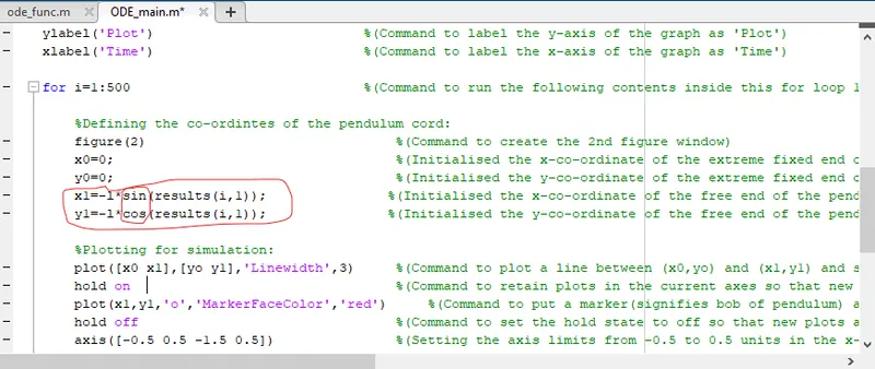
Output due to the error:
*Click on the link*:https://drive.google.com/file/d/1A-TnW80ZiFIy87__048RdKjsZrt1J3II/view?usp=sharing
We get this weird simulation where the pendulum even makes a 360o rotation.
Correction made: Instead of putting the syntax for calculating trigonometric functions in radians, I put the syntax for calculating trigonometric function in degrees.
x1=-l*sind(results(i,1));
y1=-l*cosd(results(i,1));
Error 3: Not writing ‘hold off’ command after plotting the pendulum bob (represented as a red circle) at the required position(x1,y1).
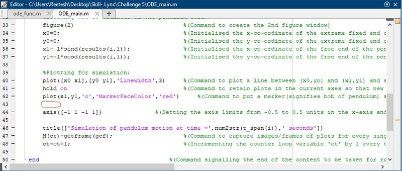
I didn’t write the ‘hold off’ command after plotting pendulum bob at the free end of the pendulum cord.
Output due to the error:
*Click on the link*:https://drive.google.com/file/d/1fyBsi1Xr0JuRGBJ25kFJ2Fdj4ER8Whlu/view?usp=sharing
As can be seen from the simulation the position of the link and the bob still remains imprinted even after the loop has finished running and the next loop has finished running. Therefore all the positions of the loop and the bob (for each and every time) still remains imprinted even after termination of the loop.
Correction made:
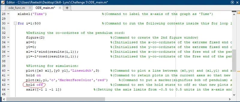
I have wrote the hold off command after plotting the pendulum bob(represented as a red circle) at the required position(x1,y1).
Error 4: While using a MATLAB function named VideoWriter I wrote Videowriter instead of VideoWriter. It threw an error on running the program as MATLAB is a case sensitive programming language and i.e. the if the same name written in ways such that if at least one of the letters differ in letter case(in 1 case it is uppercase and in another case, it is lowercase) then the two names are considered to be distinct.
In my mistake, I wrote the ‘W’ of VideoWriter function in lower case instead of uppercase.
Mistake made: (see Editor Window) and the error thrown (see Command Window): error4
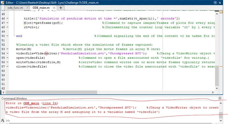
The simulation will run fine but the animation video will not be made.
Correction made: Changed the ‘W’ of VideoWriter from ‘w’ to ‘W’
CONLUSION:
- MATLAB is a great programming language and a platform to understand, analyse, simulate dynamics of any moving body or it’s components.
- A simple damped pendulum is one such moving body where we can use MATLAB to simulate its motion.
- We can also analyse the motion via the simulation and graphs (angular velocity/displacement against time) and make required conclusions necessary for putting the pendulum into use.
- Yesterday’s engineer spent a major portion of his or her time substituting values into the formulas and obtaining numerical results. However, formula manipulations and number crunching are now being left mainly to computers. Tomorrow’s engineer will need a clear understanding and a firm grasp of the basic principles so that he or she can understand even the most complex problems, formulate them, and interpret the results. MATLAB is one such fundamental tool which aids and will continue to aid tomorrow’s engineers.