Braking Energy for a given Drive Cycle & Torque-Speed Characteristics Simulation for a Lynch Motor.

OBJECTIVES:

1. To answer the question: For a defined driving cycle, calculate the energy required for braking.
2. To answer the question: Why electric motor can’t develop braking torque at high speed similar to starting? How electric and mechanical brakes are coordinated?
3. To make a MATLAB program which plots contour of given motor speed, torque and efficiency values.

SOLUTIONS:

Solution to Objective 1:

Braking: It is the process of lowering down the speed/velocity of a moving object within a given time frame or within a specific distance. During motion, the moving body has kinetic energy. In order to lower down the speed of the moving body (either to rest or to a lower speed), the kinetic energy of the body needs to be dissipated away or needs to be converted to some other form of energy.

The formula for kinetic energy present in a moving body is given by:

E _kinetic = (mv²)/2

where m -> mass of the moving object.

v -> velocity of the moving body

From the above formula, it is evident that in order to remove the kinetic energy from the moving body (assuming mass remains constant), it is necessary to reduce the velocity/speed.

Formula for the Braking Energy used for deceleration between 2 points:

Braking Energy (B.E.) = ΔK.E. = (m/2) X [(v­_i)²-(v_f)²]

where v_i -> Initial velocity

v_f -> Final Velocity

Data for a Drive Cycle defined by me is given below:

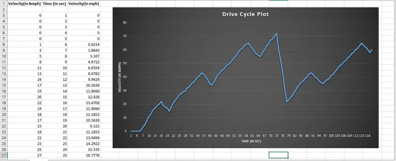
Link For the Excel Sheet:https://docs.google.com/spreadsheets/d/15hz2AfU4ZDThNwexJOGie7pPpooP-5KA/edit?usp=sharing&ouid=117524857913446184445&rtpof=true&sd=true

Now the data is loaded to the MATLAB:

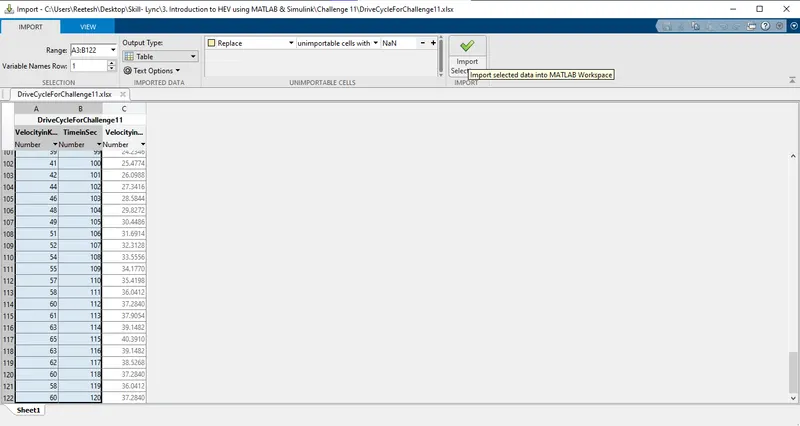
Importing the data in the Excel File to the MATLAB Workspace

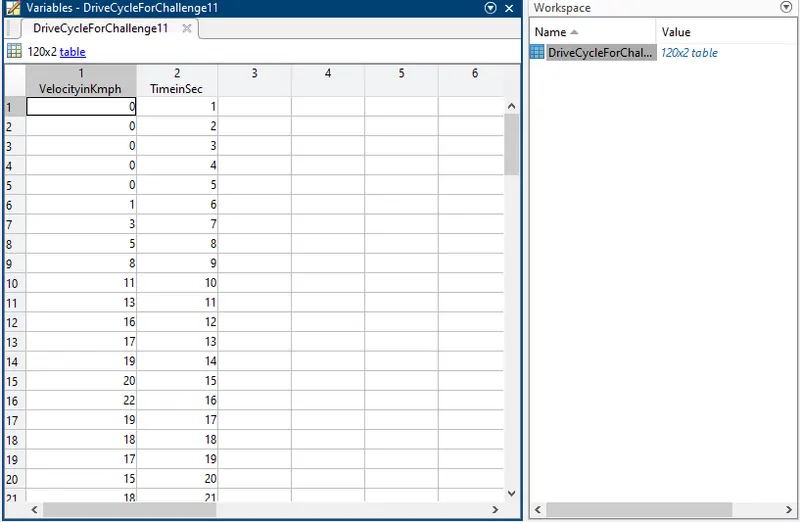
Data imported to MATLAB Workspace

My code for calculating the Total Braking Energy used, Average Braking Energy used and for plotting the Drive Cycle, Braking Energy used/time interval, Total Braking Energy after every given time interval:

close all 
clc

m=1500;                                     %Initialising the mass of the vehicle to 1500 kg
VelInKmph=DriveCycleForChallenge11{:,1};    %Extracting the Velocity values in km/hr from the Excel Sheet loaded in Workspace
VelInMs=VelInKmph*(5/18);                   %Converting the extracted velocity values from km/hr to m/s
TimeInS=DriveCycleForChallenge11{:,2};      %Extracting the Time values in seconds from the Excel Sheet loaded in Workspace
BKE=0;
BEDissip(1)=0;

for i=1:numel(TimeInS)-1                  %Implementing the for loop to calculate the Braking energy between 2 points for deceleration cases
    if VelInMs(i+1)<VelInMs(i)              %Implementing the if statement to detect cases where deceleration is occuring from initial point to final point    
        BKE=BKE+(0.5*m)*((VelInMs(i)).^2-(VelInMs(i+1)).^2);        
        BE(i)=(0.5*m)*((VelInMs(i))^2-(VelInMs(i+1))^2);      %Implementing the formula to calculate the Braking Energy for each case of deceleration
    else                                                      %Implementing the else statement to detect cases where there is acceleration/uniform velocity/rest condition  
        BE(i)=0;                                              %Assigning 0 value to Braking energy in cases where there is no deceleration  
    end                                                         %Implementing the end statement to indicate the termination of 'if' statement
    TimeDiff(i)=TimeInS(i+1)-TimeInS(1);                        %Assigning the Time Interval values between which Braking Energy was used/not used
    if i~=1
    BEDissip(i)=BEDissip(i-1)+BE(i);                            %Calculating the Net Braking Energy spent from the begining after every iteration
    end
end                                                             %Implementing the end statement to indicate the termination of 'for' statement

fprintf('Total Braking Energy used is: %d J',sum(BE));               %Command to display the net Braking Energy used in the Command Window
fprintf('nAverage Braking Energy used is: %d J',mean(BE));          %Command to display the Average Braking Energy used in the Command Window

%Plot to show the Braking Energy used for a given time interval: 
figure(1)
plot(TimeDiff,BE,'Linewidth',2)
xlabel('Time Interval in seconds')
ylabel('Braking Energy in J')
title('Braking Energy used per iteration')
grid on

%Plot to show the Drive Cycle Plot:
figure(2)
plot(TimeInS,VelInMs,'Linewidth',2)
xlabel('Time in seconds')
ylabel('Vehicle Velocity in m/s')
title('Drive Cycle Plot')
grid on

%Plot to show the total Braking Energy dissipated for a given number of iterations: 
figure(3)
plot(TimeDiff,BEDissip,'Linewidth',2)
xlabel('Time Interval in seconds')
ylabel('Braking Energy Dissipated in J')
title('Total Braking Energy Dissipated after every iteration')
grid on

Outputs Obtained:

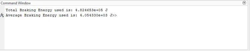
Result dispayed on Command Window after running the code

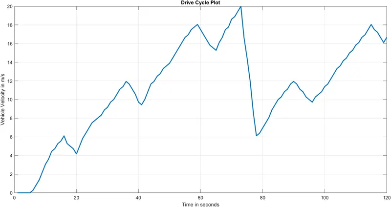
Drive Cycle Plot Obtained on running the code

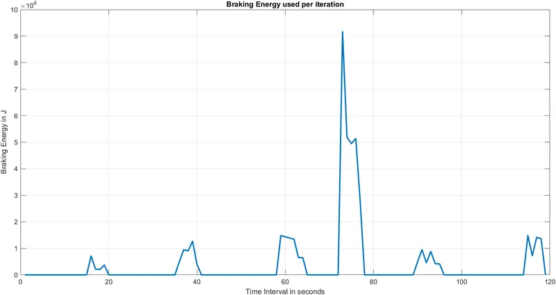
Braking Energy used for a given Time Interval for the Drive Cycle

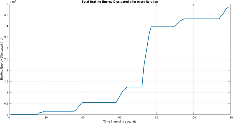
Total Braking Energy used up after every given Time Interval

Solution to Objective 2:

Braking Torque: Braking Torque is the negative torque or the torque generated on rotating in opposite direction to that of rotor rotation during acceleration or motoring.

Starting Torque: Starting Torque is the torque that an electrical motor develops when starting at zero speed.

In Torque-Speed characteristics of an electric motor, the high speed region corresponds to the region where the motor operates at a speed greater than its rated speed. This region is also known as the constant power region.

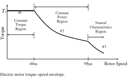
Torque-Speed envelope for an Electric Motor

Let the electric motor under consideration be an Induction Motor. The steady-state torque Characteristics of an Induction Motor is given below:

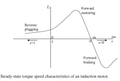
Steady state Torque-Speed characteristics of an Induction Motor

The motor always operates in the linear region of the Torque-Speed curve to avoid higher losses associated with high slip operation. As shown in the curve, the starting point of the linear portion of the curve roughly corresponds to the rated speed of the motor which also indicates the start of the high speed-region of the motor operation.

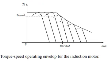
Torque-Speed Operating envelop for Induction Motor for various frequencies

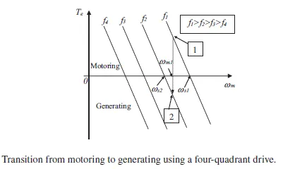
Picture depicting the transition from motoring to generating. Point 1 indicates the point where Brakes are applied and point 2 indicates the point from where deceleration of the vehicle will start occuring

In this high speed region, suppose the driver applies the brakes to slow down the vehicle. On application of brakes, the vehicle system controller lowers the motor drive frequency (operating) such that that motor speed becomes greater than synchronous speed at the newly lowered frequency. Thus, for the same rotor speed, the new operating point in the Forward Braking Region (negative torque, positive speed quadrant) has a torque value lesser than the starting torque as well as lesser than the torque value of the previous operating point in the Forward motoring region (Positive Torque, Positive Speed quadrant) before which the Brakes were applied. At this new operating point, the slip and the electromagnetic torque are negative and the motor is regenerating. Hereon, from this condition, the vehicle will decelerate. As the rotor speed decreases and goes below the synchronous speed, the operating frequency of motor again needs to be changed to a lower value so that the generating mode can be maintained. This phenomenon of generating/regenerative braking continues as long as there is kinetic energy available and the driver wishes to slow down the vehicle.

Co-ordination of Mechanical Brake and Electric Brakes:

In EVs, HEVs and FCVs, it is mandatory for mechanical friction braking systems to co-exist with electrical regenerative braking system. It is mandatory because the braking torque required is much larger than what an electric motor can produce, especially for heavy braking. The final goal of such hybrid Braking systems is not only to ensure optimum & stable braking performance but also recover as much braking energy as possible.

Usually, regenerative braking is effective only for the drive axle (front axle in most vehicles). In the speed range in which the braking energy is most dissipated, the operating efficiency of the electric motor acting as a generator is given top priority. In other speed ranges (low speed ranges), regenerative braking may be abandoned with no significant compromise on energy recovered because in such speed ranges it becomes difficult to regenerate because of the low emf generated at low rotor rotational speeds.

It should be noted that the rotational speed of a vehicle’s drive wheels, which is proportional to the motor angular speed, is decoupled from the translational speed of the vehicle body when the vehicle’s wheels are close to being locked. Thus, the operation of a hybrid brake system must be at speeds higher than a minimum threshold value. Electric regenerative braking should be applied primarily to recapture as much braking energy as possible. At speeds lower than this threshold, mechanical braking should be primarily applied to ensure the vehicle’s braking performance. Thus in low speed ranges, mechanical brakes are generally used for braking.

At higher speeds, the mechanical brakes are coupled with electric brakes as electric brakes alone cannot meet the requirements of braking energy required to bring the vehicle back to rest or a very low velocity. This is because the electric motor does not produce sufficient braking torque which it can produce during acceleration (from rest). Thus to compensate for the limits of electric brakes in stopping a vehicle, mechanical brakes are used.

Solution to Objective 3:

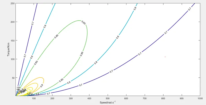
Objective of the code: To generate the operating regions of Torque-Speed Characteristics for given sets of working efficiency of a Lynch motor taking into considerations the losses involved during its operation.

In general, following are the losses involved in the working of any general electric motor (Including Lynch Motor):

• Copper losses: This losses take place due to the resistance in the armature of the motor.

Energy Loss due to Copper Loss = I_a²R_a = K_cT²

where I_a -> Current flowing in the Armature

R_a -> Resistance in the armature

K_c -> Constant which takes into account the resistance of brushes/coil, magnetic field and effect.

T -> Torque generated by the motor.

• Iron Losses: This losses take place in the armature core of the rotor. Since the armature core is made of iron and it rotates in a magnetic field, a small amount of current gets induced in the core itself too. Due to this current, eddy current loss and hysteresis loss occur in the armature iron core. Iron losses are also called as Core losses or magnetic losses.

Energy Loss due to Iron Loss = K_iω

K_i -> This constant takes into account the effects of magnetic field

ω -> Angular speed of the rotor

• Windage Losses: These losses due to air friction acting on the rotating armature.

Energy Loss due to Windage Loss = K_wω³

K_w -> Constant which takes into consideration the size and shape of the armature.

ω -> Angular Speed of the rotor.

• Other Losses: This takes into account the other losses apart from the 3 losses mentioned above which occur during the motor operation.

Energy Loss due to the other losses = C

C -> Predefined constant which takes into account the other energy losses apart from the 3 losses mentioned above.

My code to plot the Motor Speed-Torque-Efficiency contour lines:

clear
close all
clc

%Initialising a range of Speed and Torque values:
Vel=linspace(1,1000);           %Initialising a range of Velocity values
Tor=linspace(1,250);            %Intialising  range of Torque values

%Initialising the Loss Constants for calculating the Losses:
kc=0.2;                         %Initialising the constant for calculating Copper losses
ki=0.008;                       %Initialising the constant for calculating Iron losses
kw=0.0001;                      %Initialising the constant for calculating Windage losses
ConL=20;                        %Initialsing the constant value as a subsitute for other losses

[S,T]=meshgrid(Vel,Tor);        %Meshing the Speed-Torque vector values as 2-D co-ordinates with Velocity/Speed as x co-ordinate and Torque as the y co-ordinate
OutputPower=(S.*T);             %Implementing the formula to calculate the Output Power based on Speed and its corresponding Torque value 

%Calculating the Losses:
CopLoss=(T.^2)*kc;              %Calculating the Energy Loss due to Copper Loss
IronLoss=S.*ki;                 %Calculating the Energy Loss due to Iron Loss
WLoss=(S.^3)*kw;                %Calculating the Energy Loss due to Windage Loss

%Caluclating the Output Power and Efficiency:
InputPower=OutputPower+CopLoss+IronLoss+WLoss;      %Implementing the Formula to calculate the Input Power supplied by the motor
Eff=OutputPower./InputPower;                        %Implementing the Formula to calculate the Efficiency of the motor


EffDefine=[0.70,0.80,0.85,0.90,0.91,0.92,0.925,0.93];       %Specifying the z-axis/Efficiency values for which the contour lines will be shown

%Plotting the Contour Lines with Speed as the x co-ordinate, Torque as the y co-ordinate and Efficiency as the z co-ordinate:
contour(S,T,Eff,EffDefine,'ShowText','on','Linewidth',2);       %Command to plot the contour lines
box off;
grid on;
xlabel('Speed/rad.s^-^1')       %Labelling the x-axis which corresponds to the Motor Speed     
ylabel('Torque/N.m');           %Labelling the y-axis which corresponds to the Torque

The contour plot lines obtained are as follows: