Curve Fitting using MATLAB Scripting
AIM:
- To write a code in MATLAB to fit a linear and cubic polynomial for the Molar Heat Capacity data as given in the file attached with the question which shows the value of Molar Heat Capacity for each Temperature value.
- To plot the linear fit and cubic fit along with the curve joining raw data points.
- To fit a linear and cubic polynomial for the same data set by splitting the data into two and then applying the linear and cubic fit for each split part.
- To measure and compare the fitness characteristics for the curves:
- Linear Polynomial Fit on whole data set.
- Cubic Polynomial fit on whole data set.
- Whole data set divided into parts and linear polynomial fit applied to each part(Split wise method)
- Whole data set divided into parts and cubic polynomial fit applied to each part (Split wise method).
GOVERNING EQUATIONS AND RELEVANT THEORY:
- Curve Fitting is the process of constructing a curve or a mathematical function that best fits to a series of data points (co-ordinates on a plane/space).
- Curve Fitting is often used to find out an approximate relationship (mathematical function) between the independent variable(s) and the dependent variable, given a set of data points on an (independent variable(s)-dependent variable) plane/space.
- Using this approximate relationship (mathematical function), we can find out the trend of the data set and further predict new data points on the same (independent variable(s)-dependent variable) plane/space.
- For this project, I will be writing a code to fit a series of data points where each data point signifies a particular value of Molar Heat Capacity for a particular value of Temperature.
- For my curve fitting project, I will be using polynomial functions to curve fit the data points.
- Polynomial function are of the form:

Where f(x) is a polynomial function of order ‘n’.
- For my project, I will be using the polynomial fit of 1st order (Linear fit) and polynomial fit of 3rd order (Cubic fit) to fit the data points.
- After curve fitting the data points, I will be analysing the quality (accuracy & precision) of the curve fit by measuring the fitness characteristics of the particular curve fit:
The quantities used for measuring the goodness of the curve fit are:
- Sum of Squares of Error (S.S.E.): In this quantity, the difference between the data point and the curve fitted data for the same value of Independent variable is measured and squared. This is done for all mentioned values of independent variable and at the end their sum is taken. This sum gives the value of S.E. The formula of S.S.E. is:

where i =value of independent variable.
Y(i)=value of dependent variable for the given value independent variable ‘i’ as per the given data points.
f(x(i))=value of dependent variable for the given value of independent variable ‘i’ as per the function of curve fit.
But in order to evaluate the goodness of fit using this quantity, we need to know the function of the curve fit. We know the order of the function to be used for curve fit but we don’t know the values of the unit less coefficients of the polynomial function used for curve fit.
Let the polynomial function used for the curve fit be:
Where f(x) is a polynomial function of order ‘n’.
We can find out the value of the coefficients a0, a1, a2, ……. , an by differentiating the value of S.S.E. w.r.t. each and every coefficient(one at a time) and equate them to 0.
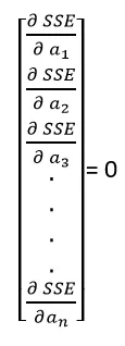
We have n equations with n unknowns. Therefore, we can solve and find out the value of all the coefficients and get the function of the curve fit with all the coefficients known.
Calculation of S.S.E. involves measuring the distance between the data point and the curve fit function. The lower the distance, better the fit of the curve and thus lesser the value of S.S.E.
- R-Squared: R-squared (R2) is popular as a statistical measure that represents the proportion of the variance for a dependent R-squared explains to what extent the variance of one variable explains the variance of the second one. So, if the R2 value of a model is 0.50, then approximately half of the observed variation will be explained by its inputs.
R Squared is also known as the coefficient of determination and represented by R² or r² and pronounced as R Squared. It is the number indicating the variance in the dependent variable that is predicted from the independent variable.
Let us consider the following diagram:
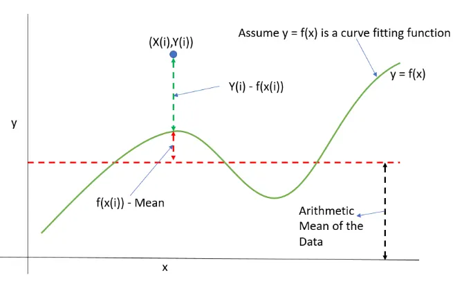
Image source: 1582722183.png (655×413) (edxengine-projects-files.s3.amazonaws.com)
In the above diagram, the data point (X(i),Y(i)),the curve fitting function y=f(x) and the arithmetic mean of the original data points is represented.
There is a quantity called SSR (Sum of squares of regression) needed to calculate the R-squared. For calculating SSR, we need to arithmetic mean of the original data points which is given by:
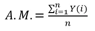
Where n=no. of data points
Y (i) =value of dependent variable for the given value independent variable ‘i’ as per the given data points.
A.M. = Arithmetic mean of original data points.
Now, S.S.R. is given by:
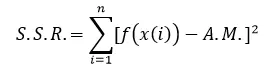
where
f(x(i))=value of dependent variable for the given value of independent variable ‘i’ as per the function of curve fit.
Now the value of R-Squared for the data set is given by:
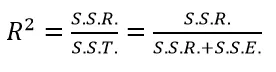
where S.S.T.=Sum of Squared Total.
From the above formula it is evident that the range of R2 is [0,1]:
- The value of R2 is 0 when S.S.R.=0. This indicates that the curve fit applied for the data set is the worst possible curve fit for the data set.
- The value of R2=1 when S.S.E.=0. This indicates that the curve fit applied for the data set is the best possible curve fit for the data set.
Therefore, we can conclude that as R2 tends to 0, the curve fit gets poorer and as R2 tends to 1, the curve fit gets better.
- Root Mean Square Error: It is another parameter that is used to measure the goodness of curve fit. Root Mean Square Error (RMSE) is the standard deviation of the residuals (prediction errors). Residuals are a measure of how far from the curve fit data points are from the original data points. RMSE is a measure of how spread out these residuals are. In other words, it tells you how concentrated the data is around the line of best fit.
The formula for R.S.M.E. is given by:
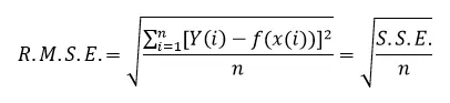
where S.S.E.=Sum of Squared Error.
n=no. of data points.
BODY OF THE CONTENT:
- Programming Language used: MATLAB
- Attached below is my entire code:
clear
close all
clc

%Preparing data:
cp_data=load('data');
temperature=cp_data(:,1);
cp=cp_data(:,2);
temperature1=cp_data(1:(end/2),1);
cp1=cp_data(1:(end/2),2);
temperature2=cp_data((end/2)+1:(end),1);
cp2=cp_data((end/2)+1:(end),2);

%1. Linear Fit on whole data set:

%1.1 Plot Molar Heat Capacity vs Temperature(Whole):
figure(1)
plot(temperature,cp,'linewidth',5)
xlabel('Temperature')
ylabel('Molar Heat Capacity')

%Linear Curve Fit(whole):
%c_p=(a*T)+b
LinWholeCo_effs=polyfit(temperature,cp,1);
Predicted_CpLinWhole=polyval(LinWholeCo_effs,temperature);

%Compare my curve fit(Linear(whole)) with original data(whole):
hold on
plot(temperature,Predicted_CpLinWhole,'linewidth',2)
legend('Original Data set','Curve Fit(Linear)')
title('Linear Polynomial fit on (Molar Heat capacity vs Temperature) data points')

%1.2
%Measuring SSE error between curve fit(Linear(whole)) and original data(whole):

EachSseLinWhole=0;
for i=1:(numel(cp_data)/2)
    Error_SseLinWhole(i)=(cp(i)-Predicted_CpLinWhole(i))^2;
    EachSseLinWhole=EachSseLinWhole+Error_SseLinWhole(i);
    SumSseLinWhole(i)=EachSseLinWhole;
end
SseLinWhole=SumSseLinWhole(end);

%Plotting Sum of Squared Error (Linear(whole)) w.r.t. Temperature:
figure(2)
plot(temperature,Error_SseLinWhole,'Linewidth',3)
xlabel('Temperature')
ylabel('Squared Error(calculated for linear fit on whole data)')
title('Variation of Squared Error(calculated for Linear fit on whole data) w.r.t. Temperature')

%1.3
%Measuring R-Sqaured (Linear(whole)) w.r.t. Temperature:
EachSsrLinWhole=0;
am=sum(cp)/numel(temperature);
for i=1:(numel(cp))
    Error_SsrLinWhole(i)=(cp(i)-am)^2;
    EachSsrLinWhole=EachSsrLinWhole+Error_SsrLinWhole(i);
    SumSsrLinWhole(i)=EachSsrLinWhole;
    Each_R_squareLinWhole(i)=Error_SseLinWhole(i)/(Error_SseLinWhole(i)+Error_SsrLinWhole(i));
    Sum_R_squareLinWhole(i)=SumSsrLinWhole(i)/(SumSseLinWhole(i)+SumSsrLinWhole(i));
end
R_squareLinWhole=Sum_R_squareLinWhole(end);

%Plotting R-squared value (Linear(whole)) w.r.t. Temperature:
figure(3)
plot(temperature,Each_R_squareLinWhole,'Linewidth',3)
xlabel('Temperature')
ylabel('Squared Error/(Squared Error + Squared Regression)')
title('Variation of [Squared Error/(Squared Error + Squared Regression)](calulated for Linear fit on whole data) w.r.t. Temperature')

%1.4
%Measuring Root Mean Square Error between data points & Curve fit(Linear(whole)):

for i=1:(numel(cp))
    Each_RmseLinWhole(i)=sqrt(Error_SseLinWhole(i)/i);
    Sum_RmseLinWhole(i)=sqrt(SumSseLinWhole(i)/i);
end
RMSELinWhole=Sum_RmseLinWhole(end);

%Plotting Root Mean Squared Error(Linear(whole)) w.r.t. Temperature:
figure(4)
plot(temperature,Sum_RmseLinWhole,'Linewidth',3)
xlabel('Temperature')
ylabel('Root Mean Square Error')
title('Variation of R.M.S.E.(calculated for Linear Fit on whole data) w.r.t. Temperature')


%2.Cubic Fit on whole Data Set:

%2.1
%Plot Molar Heat Capacity vs Temperature(Whole):
figure(5)
plot(temperature,cp,'linewidth',5)
xlabel('Temperature')
ylabel('Molar Heat Capacity')

%Cubic Curve Fit(whole):
%c_p=(a*T^3)+(b*T^2)+(c*T)+d:
CubeWholeCo_effs=polyfit(temperature,cp,3);
Predicted_CpCubeWhole=polyval(CubeWholeCo_effs,temperature);

%2.2
%Compare my curve fit(Cubic(whole)) with original data(whole):
hold on
plot(temperature,Predicted_CpCubeWhole,'linewidth',2)
legend('Original Data set','Curve Fit(Cubic)')
title('Cubic polynomial fit on (Molar Heat capacity vs Temperature) data points')

%Measuring SSE error between curve fit(Cubic(whole)) and original data(whole):
EachSseCubeWhole=0;
for i=1:(numel(cp_data)/2)
    Error_SseCubeWhole(i)=(cp(i)-Predicted_CpCubeWhole(i))^2;
    EachSseCubeWhole=EachSseCubeWhole+Error_SseCubeWhole(i);
    SumSseCubeWhole(i)=EachSseCubeWhole;
end
SseCubeWhole=SumSseCubeWhole(end);

%2.3
%Plotting Sum of Squared Error(Cubic regression(whole)) w.r.t. Temperature:
figure(6)
plot(temperature,Error_SseCubeWhole,'Linewidth',3)
xlabel('Temperature')
ylabel('Squared Error(calculated for cubic fit on whole data)')
title('Variation of Squared Error(calculated for Cubic fit on whole data) w.r.t. Temperature')

%Measuring R-Sqaured value between data points and curve fit(Cubic(whole))
EachSsrCubeWhole=0;
am=sum(cp)/numel(temperature);
for i=1:(numel(cp))
    Error_SsrCubeWhole(i)=(cp(i)-am)^2;
    EachSsrCubeWhole=EachSsrCubeWhole+Error_SsrCubeWhole(i);
    SumSsrCubeWhole(i)=EachSsrCubeWhole;
    Each_R_squareCubeWhole(i)=Error_SseCubeWhole(i)/(Error_SseCubeWhole(i)+Error_SsrCubeWhole(i));
    Each_R_squareCubeWhole(i)=SumSsrCubeWhole(i)/(SumSseCubeWhole(i)+SumSsrCubeWhole(i));
end
R_squareCubeWhole=Each_R_squareCubeWhole(i);

%Plotting R-squared value (Linear(whole)) w.r.t. Temperature:
figure(7)
plot(temperature,Each_R_squareCubeWhole,'Linewidth',3)
xlabel('Temperature')
ylabel('Squared Error/(Squared Error + Squared Regression)')
title('Variation of [Squared Error/(Squared Error + Squared Regression)](calulated for Linear fit on whole data) w.r.t. Temperature')

%2.4
%Measuring Root Mean Square Error between data points & Curve fit(Linear(whole)):
for i=1:(numel(cp))
    Each_RmseCubeWhole(i)=sqrt(Error_SseCubeWhole(i)/i);
    Sum_RmseCubeWhole(i)=sqrt(SumSseCubeWhole(i)/i);
end
RMSECubeWhole=Sum_RmseCubeWhole(end);

%Plotting Root Mean Squared Error(Linear(whole)) w.r.t. Temperature:
figure(8)
plot(temperature,Sum_RmseCubeWhole,'Linewidth',3)
xlabel('Temperature')
ylabel('Root Mean Square Error')
title('Variation of R.M.S.E.(calculated for Cubic Fit on whole data) w.r.t. Temperature')


%3.Linear Fit on Split Data Set:

%3.1
%Plot Molar Heat Capacity vs Temperature(Splitwise 2 halves for Linear Fit):
figure(9)
plot(temperature1,cp1,'linewidth',5)
hold on
plot(temperature2,cp2,'linewidth',5)
xlabel('Temperature[K]')
ylabel('Molar Heat Capacity[KJ/kmol-K]')

%Linear Curve Fit(Split-wise into 2 halves):
%c_p=(a*T)+b
LinSplitCo_effs1=polyfit(temperature1,cp1,1);
LinSplitCo_effs2=polyfit(temperature2,cp2,1);
Predicted_CpLinSplit1=polyval(LinSplitCo_effs1,temperature1);
Predicted_CpLinSplit2=polyval(LinSplitCo_effs2,temperature2);

%Compare my curve fit(linear(spit into 2 halves)) with original data(Split-wise into 2 halves):
hold on
plot(temperature1,Predicted_CpLinSplit1,'linewidth',2,'color','y')
plot(temperature2,Predicted_CpLinSplit2,'linewidth',2,'color','g')
title('Variation of Molar Heat Capacity w.r.t. Temperature')
legend('Original Data Set 1st half','Original Data Set 2nd half','Linear Fit 1st half','Linear Fit 2nd half')
hold off

%3.2
%Measuring SSE Error between curve fit(linear) and original data(Split-wise into 2 halves):
Each1SseLinSplit=0;
Each2SseLinSplit=0;
for i=1:(numel(cp_data)/4)
    Error1_SseLinSplit(i)=(cp1(i)-Predicted_CpLinSplit1(i))^2;
    Error2_SseLinSplit(i)=(cp2(i)-Predicted_CpLinSplit2(i))^2;
    Each1SseLinSplit=Each1SseLinSplit+Error1_SseLinSplit(i);
    Each2SseLinSplit=Each2SseLinSplit+Error2_SseLinSplit(i);
    Sum1SseLinSplit(i)=Each1SseLinSplit;
    Sum2SseLinSplit(i)=Each2SseLinSplit;
    SumSseLinSplit(i)=Sum1SseLinSplit(i)+Sum2SseLinSplit(i);
end
SseLinSplit=SumSseLinSplit(end);

%Plotting Sum of Squared Error(Cubic splitwise) w.r.t. Temperature:
figure(10);
plot(temperature1,Error1_SseLinSplit,'linewidth',3)
hold on
plot(temperature2,Error2_SseLinSplit,'linewidth',3)
xlabel('Temperature')
ylabel('Squared Error(calculated for Linear Fit on Split Data)')
title('Variation of Squared Error(calculated for Linear fit on split data) w.r.t. Temperature')
legend('Squared Error of 1st half of data set','Squared Error of 2nd half of data set')

%3.3
%Measuring R-squared Error between curve fit(linear) and original data(split into 2 halves):
Each1_SsrLinSplit=0;
Each2_SsrLinSplit=0;
am1=sum(cp1)/numel(temperature1);
am2=sum(cp2)/numel(temperature2);
for i=1:(numel(cp1))
    Error1_SsrLinSplit(i)=(cp1(i)-am1)^2;
    Error2_SsrLinSplit(i)=(cp2(i)-am2)^2;
    Each1_SsrLinSplit=Each1_SsrLinSplit+Error1_SsrLinSplit(i);
    Each2_SsrLinSplit=Each2_SsrLinSplit+Error2_SsrLinSplit(i);
    Sum1SsrLinSplit(i)=Each1_SsrLinSplit;
    Sum2SsrLinSplit(i)=Each2_SsrLinSplit;
    SumSsrLinSplit(i)=Sum1SsrLinSplit(i)+Sum2SsrLinSplit(i);
    Each1_R_squareLinSplit(i)=Error1_SsrLinSplit(i)/(Error1_SseLinSplit(i)+Error1_SsrLinSplit(i));
    Each2_R_squareLinSplit(i)=Error2_SsrLinSplit(i)/(Error2_SseLinSplit(i)+Error2_SsrLinSplit(i));
    Sum1_R_squareLinSplit(i)=Sum1SsrLinSplit(i)/(Sum1SsrLinSplit(i)+Sum1SseLinSplit(i));
    Sum2_R_squareLinSplit(i)=Sum2SsrLinSplit(i)/(Sum2SsrLinSplit(i)+Sum2SseLinSplit(i));
    Sum_R_squareLinSplit(i)=SumSsrLinSplit(i)/(SumSsrLinSplit(i)+SumSseLinSplit(i));
end
R_squareLinSplit=Sum_R_squareLinSplit(end);

%Plotting R-squared Error(Cubic Splitwise) w.r.t. Temperature:
figure(11);
plot(temperature1,Each1_R_squareLinSplit,'linewidth',3)
hold on
plot(temperature2,Each2_R_squareLinSplit,'linewidth',3)
xlabel('Temperature')
ylabel('Squared Error/(Squared Error + Squared Regression)')
title('Variation of [Squared Error/(Squared Error + Squared Regression)](calculated for 2 halves of data set) w.r.t. Temperature')
legend('Squared Error/(Squared Error + Squared Regression) of 1st half of data set','Squared Error/(Squared Error + Squared Regression) of 2nd half of data set')

%3.4
%Measuring Root Mean Square Error between data points & Curve fit(Linear(whole)):
for i=1:(numel(cp1))
    Each1_RmseLinSplit(i)=sqrt(Error1_SseLinSplit(i)/i);
    Each2_RmseLinSplit(i)=sqrt(Error2_SseLinSplit(i)/i);
    Sum1_RmseLinSplit(i)=sqrt(Sum1SseLinSplit(i)/i);
    Sum2_RmseLinSplit(i)=sqrt(Sum2SseLinSplit(i)/i);
    Sum_RmseLinSplit(i)=sqrt((Sum1SseLinSplit(i)+Sum2SseLinSplit(i))/(i+i));
end
RMSELinSplit=Sum_RmseLinSplit(end);


%Plotting Root Mean Squared Error(Cubic(split)) w.r.t. Temperature:
figure(12)
plot(temperature1,Sum1_RmseLinSplit,'Linewidth',3)
hold on
plot(temperature2,Sum2_RmseLinSplit,'Linewidth',3)
xlabel('Temperature')
ylabel('Root Mean Square Error')
title('Variation of R.M.S.E.(calculated for Linear Fit on split data) w.r.t. Temperature')
legend('RMSE of 1st half of data set','RMSE of 2nd half of data set')

%4.Cubic Fit on Split data set:

%4.1
%Plot Molar Heat Capacity vs Temperature(Splitwise 2 halves for Cubic Fit):
figure(13)
plot(temperature1,cp1,'linewidth',5)
hold on
plot(temperature2,cp2,'linewidth',5)
xlabel('Temperature[K]')
ylabel('Molar Heat Capacity[KJ/kmol-K]')

%Cubic Curve Fit(Split-wise into 2 halves):
%c_p=(a*T^3)+(b*T^2)+(c*T)+d
CubeSplitCo_effs1=polyfit(temperature1,cp1,3);
CubeSplitCo_effs2=polyfit(temperature2,cp2,3);
Predicted_CpCubeSplit1=polyval(CubeSplitCo_effs1,temperature1);
Predicted_CpCubeSplit2=polyval(CubeSplitCo_effs2,temperature2);

%Compare my curve fit(cubic(spit into 2 halves)) with original data(Split-wise into 2 halves):
hold on
plot(temperature1,Predicted_CpCubeSplit1,'linewidth',2,'color','y')
plot(temperature2,Predicted_CpCubeSplit2,'linewidth',2,'color','g')
legend('Original Data Set 1st half','Original Data Set 2nd half','Cubic Fit 1st half','Cubic Fit 2nd half')
hold off

%4.2
%Measuring SSE Error between curve fit(cubic) and original data(Split-wise into 2 halves):
Each1SseCubeSplit=0;
Each2SseCubeSplit=0;
for i=1:(numel(cp_data)/4)
    Error1_SseCubeSplit(i)=(cp1(i)-Predicted_CpCubeSplit1(i))^2;
    Error2_SseCubeSplit(i)=(cp2(i)-Predicted_CpCubeSplit2(i))^2;
    Each1SseCubeSplit=Each1SseCubeSplit+Error1_SseCubeSplit(i);
    Each2SseCubeSplit=Each2SseCubeSplit+Error2_SseCubeSplit(i);
    Sum1SseCubeSplit(i)=Each1SseCubeSplit;
    Sum2SseCubeSplit(i)=Each2SseCubeSplit;
    SumSseCubeSplit(i)=Sum1SseCubeSplit(i)+Sum2SseCubeSplit(i);
end
SseCubeSplit=SumSseCubeSplit(end);

%Plotting Sum of Squared Error(Cubic splitwise) w.r.t. Temperature:
figure(14);
plot(temperature1,Error1_SseCubeSplit,'linewidth',3)
hold on
plot(temperature2,Error2_SseCubeSplit,'linewidth',3)
xlabel('Temperature')
ylabel('Squared Error(calculated for Cubic Fit on Split Data)')
title('Variation of Squared Error(calculated for Cubic Regression on split data) w.r.t. Temperature')
legend('Squared Error of 1st half of data set','Squared Error of 2nd half of data set')

%4.3
%Measuring R-squared Error between curve fit(cubic) and original data(split into 2 halves):
Each1_SsrCubeSplit=0;
Each2_SsrCubeSplit=0;
am1=sum(cp1)/numel(temperature1);
am2=sum(cp2)/numel(temperature2);
for i=1:(numel(cp1))
    Error1_SsrCubeSplit(i)=(cp1(i)-am1)^2;
    Error2_SsrCubeSplit(i)=(cp2(i)-am2)^2;
    Each1_SsrCubeSplit=Each1_SsrCubeSplit+Error1_SsrCubeSplit(i);
    Each2_SsrCubeSplit=Each2_SsrCubeSplit+Error2_SsrCubeSplit(i);
    Sum1SsrCubeSplit(i)=Each1_SsrCubeSplit;
    Sum2SsrCubeSplit(i)=Each2_SsrCubeSplit;
    SumSsrCubeSplit(i)=Sum1SsrCubeSplit(i)+Sum2SsrCubeSplit(i);
    Each1_R_squareCubeSplit(i)=Error1_SsrCubeSplit(i)/(Error1_SseCubeSplit(i)+Error1_SsrCubeSplit(i));
    Each2_R_squareCubeSplit(i)=Error2_SsrCubeSplit(i)/(Error2_SseCubeSplit(i)+Error2_SsrCubeSplit(i));
    Sum1_R_squareCubeSplit(i)=Sum1SsrCubeSplit(i)/(Sum1SsrCubeSplit(i)+Sum1SseCubeSplit(i));
    Sum2_R_squareCubeSplit(i)=Sum2SsrCubeSplit(i)/(Sum2SsrCubeSplit(i)+Sum2SseCubeSplit(i));
    Sum_R_squareCubeSplit(i)=SumSsrCubeSplit(i)/(SumSsrCubeSplit(i)+SumSseCubeSplit(i));
end
R_squareCubeSplit=Sum_R_squareCubeSplit(end);

%Plotting R-squared Error(Cubic Splitwise) w.r.t. Temperature:
figure(15);
plot(temperature1,Each1_R_squareCubeSplit,'linewidth',3)
hold on
plot(temperature2,Each2_R_squareCubeSplit,'linewidth',3)
xlabel('Temperature')
ylabel('Squared Error/(Squared Error + Squared Regression)')
title('Variation of [Squared Error/(Squared Error + Squared Regression)](calculated for 2 halves of data set) w.r.t. Temperature')
legend('Squared Error/(Squared Error + Squared Regression) of 1st half of data set','Squared Error/(Squared Error + Squared Regression) of 2nd half of data set')

%4.4
%Measuring Root Mean Square Error between data points & Curve fit(Linear(whole)):
for i=1:(numel(cp1))
    Each1_RmseCubeSplit(i)=sqrt(Error1_SseCubeSplit(i)/i);
    Each2_RmseCubeSplit(i)=sqrt(Error2_SseCubeSplit(i)/i);
    Sum1_RmseCubeSplit(i)=sqrt(Sum1SseCubeSplit(i)/i);
    Sum2_RmseCubeSplit(i)=sqrt(Sum2SseCubeSplit(i)/i);
    Sum_RmseCubeSplit(i)=sqrt((Sum1SseCubeSplit(i)+Sum2SseCubeSplit(i))/(i+i));
end
RMSECubeSplit=Sum_RmseCubeSplit(end);


%Plotting Root Mean Squared Error(Cubic(split)) w.r.t. Temperature:
figure(16)
plot(temperature1,Sum1_RmseCubeSplit,'Linewidth',3)
hold on
plot(temperature2,Sum2_RmseCubeSplit,'Linewidth',3)
xlabel('Temperature')
ylabel('Root Mean Square Error')
title('Variation of R.M.S.E.(calculated for Cubic Fit on split data) w.r.t. Temperature')
legend('RMSE of 1st half of data set','RMSE of 2nd half of data set')- Firstly I have loaded the contents of the file ‘data’ into the MATLAB program and assigned variables to take the content inside the file ‘data’:
- cp_data takes all the content inside the file ‘data’ which is in the form of a (3200 X 2) matrix.
- temperature takes the content present in the 1st column of the main matrix present in ‘data’.
- cp takes the content present in the 2nd column of the main matrix present in ‘data’.
- cp1 takes the 1st half of the content present in the 2nd column of the main matrix present in ‘data’. It is in the form of a (1600 X 1) matrix.
- cp2 takes the 2nd half of the content present in the 2nd column of the main matrix present in ‘data’. It is in the form of a (1600 X 1) matrix.
- temperature1 takes the 1st half of the content present in the 1st column of the main matrix present in ‘data’. It is in the form of a (1600 X 1) matrix.
- temperature2 takes the 2nd half of the content present in the 1st column of the main matrix present in ‘data’. It is in the form of a (1600 X 1) matrix.
- My code can be analysed by breaking it into 4 sections:
- Again each section can be analysed by breaking it into 4 sub-sections:
- Section 1 -> My code to curve fit the original data using linear fit on the entire data and also plot the curve fit along with the raw data points. I will also determine the goodness of the curve fit by calculating the S.S.E.,R-squared and the RSME values for this fit on the original data points.
- Section 1.1 -> In this sub-section, the code is written to curve fit the original data using linear fit on the entire data set and plot the curve fit along with the original data points.
My code:
%1.1 Plot Molar Heat Capacity vs Temperature(Whole):
figure(1)
plot(temperature,cp,'linewidth',5)
xlabel('Temperature')
ylabel('Molar Heat Capacity')

%Linear Curve Fit(whole):
%c_p=(a*T)+b
LinWholeCo_effs=polyfit(temperature,cp,1);
Predicted_CpLinWhole=polyval(LinWholeCo_effs,temperature);

%Compare my curve fit(Linear(whole)) with original data(whole):
hold on
plot(temperature,Predicted_CpLinWhole,'linewidth',2)
legend('Original Data set','Curve Fit(Linear)')
title('Linear Polynomial fit on (Molar Heat capacity vs Temperature) data points')
In this code I have loaded the ‘Molar heat capacity’ and ‘Temperature’ values and written a code for single order polynomial fit for the (Molar Heat Capacity-Temperature) data set using the commands ‘polyfit’ and ‘polyval’.
Then I have plotted the obtained curve fit on the curve (formed by joining the original data set) where we can visually analyse the goodness of curve fit. The plot box has been named as Figure 1.
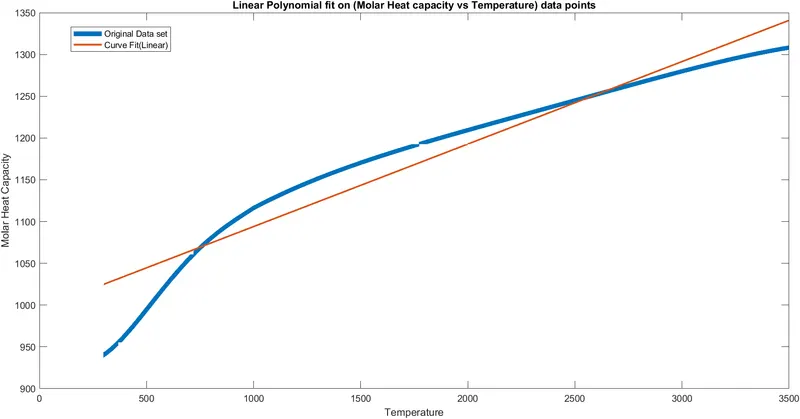
We can see that the curve fit is a poor approximation of the original data set.
- Section 1.2 -> In the second sub-section, I have written a code to calculate the S.S.E.(Sum of Squared Errors) for the obtained Linear Curve Fit and the original data set.
Attached below is my code:
%1.2
%Measuring SSE error between curve fit(Linear(whole)) and original data(whole):

EachSseLinWhole=0;
for i=1:(numel(cp_data)/2)
    Error_SseLinWhole(i)=(cp(i)-Predicted_CpLinWhole(i))^2;
    EachSseLinWhole=EachSseLinWhole+Error_SseLinWhole(i);
    SumSseLinWhole(i)=EachSseLinWhole;
end
SseLinWhole=SumSseLinWhole(end);

%Plotting Sum of Squared Error (Linear(whole)) w.r.t. Temperature:
figure(2)
plot(temperature,Error_SseLinWhole,'Linewidth',3)
xlabel('Temperature')
ylabel('Squared Error(calculated for linear fit on whole data)')
title('Variation of Squared Error(calculated for Linear fit on whole data) w.r.t. Temperature')
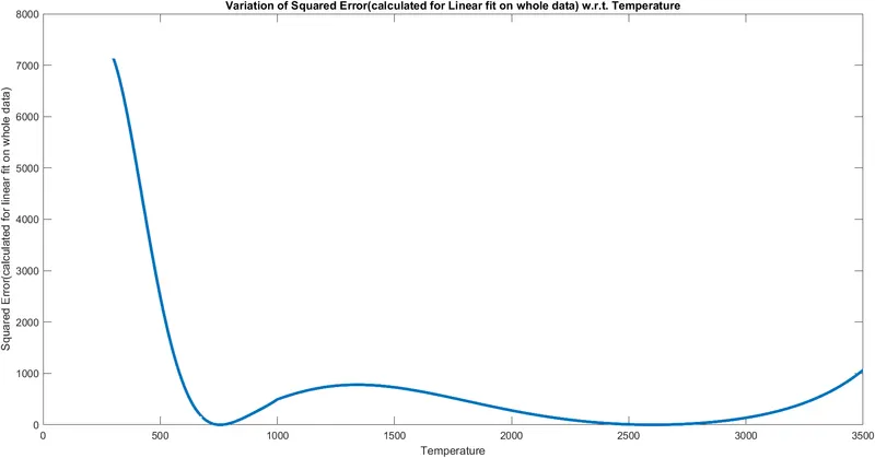
The Variable SseLinWhole will store the value of S.S.E. for the obtained Linear Curve Fit and the original data set.
In the above code I have also given commands to plot the variation of ‘Squared Error’ (not sum) for each data point w.r.t. to the corresponding value of Temperature. The plot box has been named as Figure 2.
Attached below is the plot:
- Section 1.3 -> In the third sub-section, I have written a code to calculate the R_squared value for the obtained Linear Curve Fit and the original data set.
Attached below is the code:
%1.3
%Measuring R-Sqaured (Linear(whole)) w.r.t. Temperature:
EachSsrLinWhole=0;
am=sum(cp)/numel(temperature);
for i=1:(numel(cp))
    Error_SsrLinWhole(i)=(cp(i)-am)^2;
    EachSsrLinWhole=EachSsrLinWhole+Error_SsrLinWhole(i);
    SumSsrLinWhole(i)=EachSsrLinWhole;
    Each_R_squareLinWhole(i)=Error_SseLinWhole(i)/(Error_SseLinWhole(i)+Error_SsrLinWhole(i));
    Sum_R_squareLinWhole(i)=SumSsrLinWhole(i)/(SumSseLinWhole(i)+SumSsrLinWhole(i));
end
R_squareLinWhole=Sum_R_squareLinWhole(end);

%Plotting R-squared value (Linear(whole)) w.r.t. Temperature:
figure(3)
plot(temperature,Each_R_squareLinWhole,'Linewidth',3)
xlabel('Temperature')
ylabel('Squared Error/(Squared Error + Squared Regression)')
title('Variation of [Squared Error/(Squared Error + Squared Regression)](calulated for Linear fit on whole data) w.r.t. Temperature')
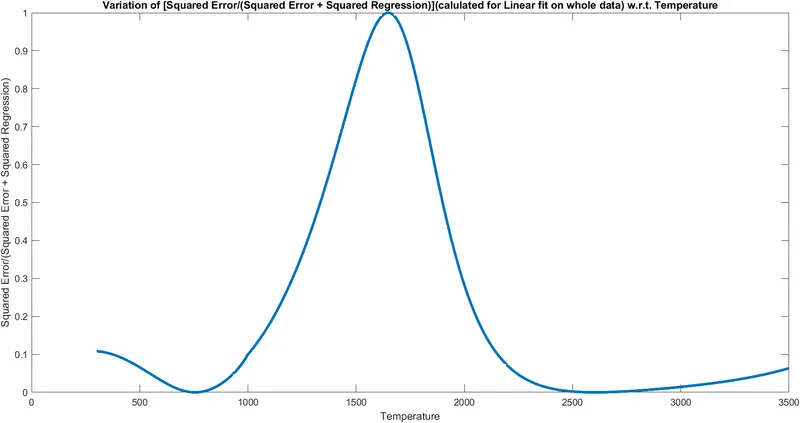
The Variable R_squareLinWhole will store the value of R-squared for the obtained Linear Curve Fit and the original data set. In the above code I have also given commands to plot the  variation of for each data point w.r.t. to the corresponding value of Temperature. The plot box has been named as Figure 3.
Attached below is the plot:
- Section 1.4 -> In the 4th sub-section, I have written a code to calculate the R.M.S.E. (Root Mean Square Error) for the obtained curve fit and the original data points.
Attached below is the code:
%1.4
%Measuring Root Mean Square Error between data points & Curve fit(Linear(whole)):

for i=1:(numel(cp))
    Each_RmseLinWhole(i)=sqrt(Error_SseLinWhole(i)/i);
    Sum_RmseLinWhole(i)=sqrt(SumSseLinWhole(i)/i);
end
RMSELinWhole=Sum_RmseLinWhole(end);

%Plotting Root Mean Squared Error(Linear(whole)) w.r.t. Temperature:
figure(4)
plot(temperature,Sum_RmseLinWhole,'Linewidth',3)
xlabel('Temperature')
ylabel('Root Mean Square Error')
title('Variation of R.M.S.E.(calculated for Linear Fit on whole data) w.r.t. Temperature')
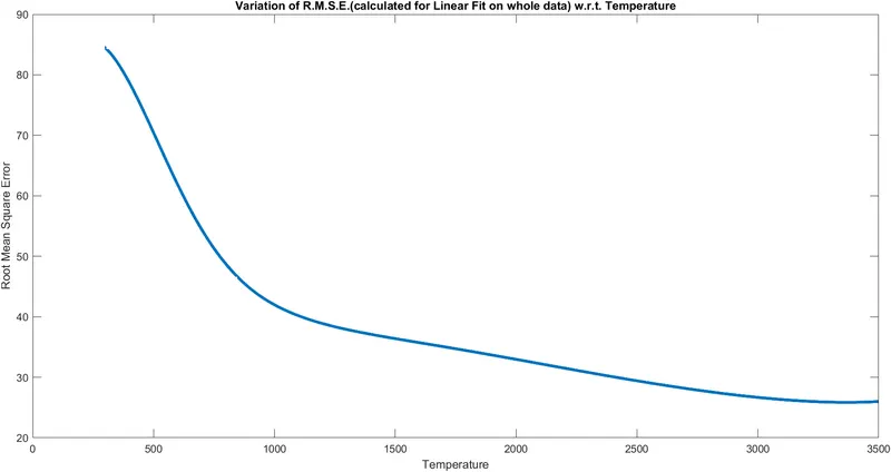
The variable RMSELinWhole will store the value of R.M.S.E. for the obtained curve fit and the original data set. In the above code, I have also given commands to plot the variation of R.M.S.E. for each data point w.r.t. to the corresponding value of temperature. The plot box has been named as Figure 4. Attached below is the plot:
- Section 2 ->This is my code to curve fit the original data using cubic fit on the entire data and also plot the curve fit along with the raw data points. I will also determine the goodness of the curve fit by calculating the S.S.E.,R-squared and the RSME values for this fit on the original data points.
- Section 2.1 -> In this sub-section, the code is written to curve fit the original data using cubic fit on the entire data set and plot the curve fit along with the original data points.
My code:
%2.1
%Plot Molar Heat Capacity vs Temperature(Whole):
figure(5)
plot(temperature,cp,'linewidth',5)
xlabel('Temperature')
ylabel('Molar Heat Capacity')

%Cubic Curve Fit(whole):
%c_p=(a*T^3)+(b*T^2)+(c*T)+d:
CubeWholeCo_effs=polyfit(temperature,cp,3);
Predicted_CpCubeWhole=polyval(CubeWholeCo_effs,temperature);

%Compare my curve fit(Cubic(whole)) with original data(whole):
hold on
plot(temperature,Predicted_CpCubeWhole,'linewidth',2)
legend('Original Data set','Curve Fit(Cubic)')
title('Cubic polynomial fit on (Molar Heat capacity vs Temperature) data points')
In this code I have loaded the ‘Molar heat capacity’ and ‘Temperature’ values and written a code for third order polynomial fit for the (Molar Heat Capacity-Temperature) data set using the commands ‘polyfit’ and ‘polyval’.
Then I have plotted the obtained curve fit on the curve (formed by joining the original data set) where we can visually analyse the goodness of curve fit. The plot box has been named as Figure 5.
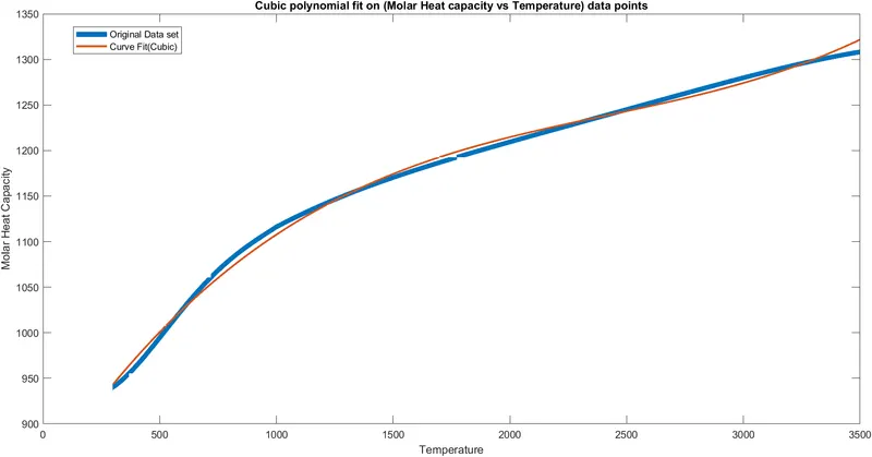
This curve fit manages to do a good job in approximation of the original data set
- Section 2.2 -> In the second sub-section, I have written a code to calculate the S.S.E.(Sum of Squared Errors) for the obtained Cubic Curve Fit and the original data set.
Attached below is my code:
%2.2
%Measuring SSE error between curve fit(Cubic(whole)) and original data(whole):
EachSseCubeWhole=0;
for i=1:(numel(cp_data)/2)
    Error_SseCubeWhole(i)=(cp(i)-Predicted_CpCubeWhole(i))^2;
    EachSseCubeWhole=EachSseCubeWhole+Error_SseCubeWhole(i);
    SumSseCubeWhole(i)=EachSseCubeWhole;
end
SseCubeWhole=SumSseCubeWhole(end);

%Plotting Sum of Squared Error(Cubic regression(whole)) w.r.t. Temperature:
figure(6)
plot(temperature,Error_SseCubeWhole,'Linewidth',3)
xlabel('Temperature')
ylabel('Squared Error(calculated for cubic fit on whole data)')
title('Variation of Squared Error(calculated for Cubic fit on whole data) w.r.t. Temperature')
The Variable SseCubeWhole will store the value of S.S.E. for the obtained Cubic Curve Fit and the original data set.
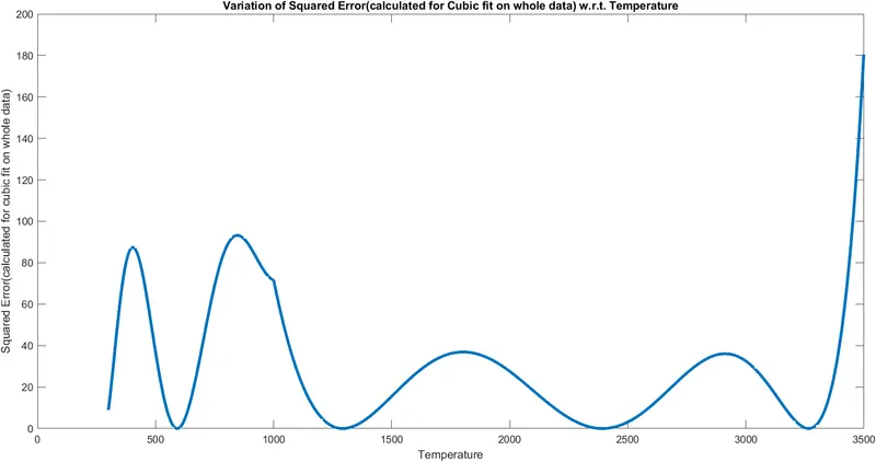
In the above code I have also given commands to plot the variation of ‘Squared Error’ (not sum) for each data point w.r.t. to the corresponding value of Temperature. The plot box has been named as Figure 6.
Attached below is the plot:
- Section 2.3 -> In the third sub-section, I have written a code to calculate the R_squared value for the obtained Linear Curve Fit and the original data set.
Attached below is the code:
%2.3
%Measuring R-Sqaured value between data points and curve fit(Cubic(whole))
EachSsrCubeWhole=0;
am=sum(cp)/numel(temperature);
for i=1:(numel(cp))
    Error_SsrCubeWhole(i)=(cp(i)-am)^2;
    EachSsrCubeWhole=EachSsrCubeWhole+Error_SsrCubeWhole(i);
    SumSsrCubeWhole(i)=EachSsrCubeWhole;
    Each_R_squareCubeWhole(i)=Error_SseCubeWhole(i)/(Error_SseCubeWhole(i)+Error_SsrCubeWhole(i));
    Each_R_squareCubeWhole(i)=SumSsrCubeWhole(i)/(SumSseCubeWhole(i)+SumSsrCubeWhole(i));
end
R_squareCubeWhole=Each_R_squareCubeWhole(i);

%Plotting R-squared value (Linear(whole)) w.r.t. Temperature:
figure(7)
plot(temperature,Each_R_squareCubeWhole,'Linewidth',3)
xlabel('Temperature')
ylabel('Squared Error/(Squared Error + Squared Regression)')
title('Variation of [Squared Error/(Squared Error + Squared Regression)](calulated for Linear fit on whole data) w.r.t. Temperature')
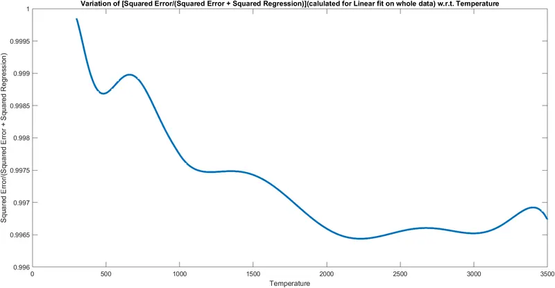
The Variable R_squareCubeWhole will store the value of R-squared for the obtained Cubic Curve Fit and the original data set. In the above code I have also given commands to plot the variation of for each data point w.r.t. to the corresponding value of Temperature. The plot box has been named as Figure 7.
Attached below is the plot:
- Section 2.4 -> In the 4th sub-section, I have written a code to calculate the R.M.S.E. (Root Mean Square Error) for the obtained cubic curve fit and the original data points.
Attached below is the code:
%2.4
%Measuring Root Mean Square Error between data points & Curve fit(Linear(whole)):
for i=1:(numel(cp))
    Each_RmseCubeWhole(i)=sqrt(Error_SseCubeWhole(i)/i);
    Sum_RmseCubeWhole(i)=sqrt(SumSseCubeWhole(i)/i);
end
RMSECubeWhole=Sum_RmseCubeWhole(end);

%Plotting Root Mean Squared Error(Linear(whole)) w.r.t. Temperature:
figure(8)
plot(temperature,Sum_RmseCubeWhole,'Linewidth',3)
xlabel('Temperature')
ylabel('Root Mean Square Error')
title('Variation of R.M.S.E.(calculated for Cubic Fit on whole data) w.r.t. Temperature')
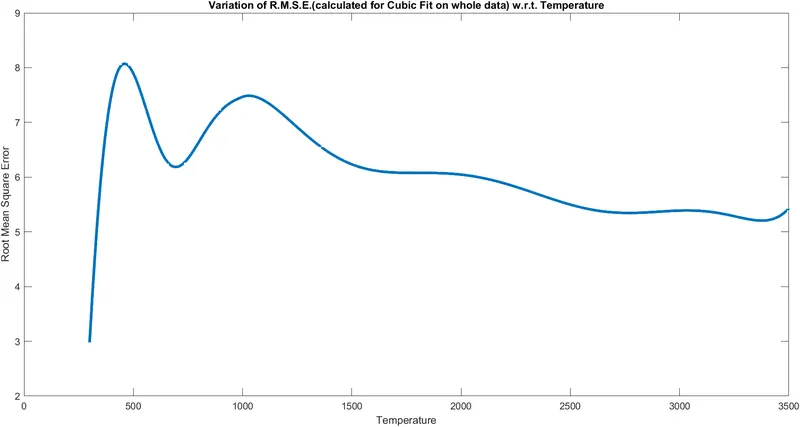
The variable RMSECubeWhole will store the value of R.M.S.E. for the obtained curve fit and the original data set. In the above code, I have also given commands to plot the variation of R.M.S.E. for each data point w.r.t. to the corresponding value of temperature. The plot box has been named as Figure 8. Attached below is the plot:
- Section 3 -> For this case, I have split my data into 2 equal halves This is my code to curve fit both the split data using linear fit on the both the data and also plot the curve fit along with the raw data points. I will also determine the goodness of both the curve fits (applied curve fit separately on each half) by calculating the S.S.E. ,R-squared and the RSME values for this fit on the original data points.
- Section 3.1 -> In this sub-section, the code is written to curve fit the original data using linear fit on each split data set and plot both curve fits along with the original data points.
My code:
%3.1
%Plot Molar Heat Capacity vs Temperature(Splitwise 2 halves for Linear Fit):
figure(9)
plot(temperature1,cp1,'linewidth',5)
hold on
plot(temperature2,cp2,'linewidth',5)
xlabel('Temperature[K]')
ylabel('Molar Heat Capacity[KJ/kmol-K]')

%Linear Curve Fit(Split-wise into 2 halves):
%c_p=(a*T)+b
LinSplitCo_effs1=polyfit(temperature1,cp1,1);
LinSplitCo_effs2=polyfit(temperature2,cp2,1);
Predicted_CpLinSplit1=polyval(LinSplitCo_effs1,temperature1);
Predicted_CpLinSplit2=polyval(LinSplitCo_effs2,temperature2);

%Compare my curve fit(linear(spit into 2 halves)) with original data(Split-wise into 2 halves):
hold on
plot(temperature1,Predicted_CpLinSplit1,'linewidth',2,'color','y')
plot(temperature2,Predicted_CpLinSplit2,'linewidth',2,'color','g')
title('Variation of Molar Heat Capacity w.r.t. Temperature')
legend('Original Data Set 1st half','Original Data Set 2nd half','Linear Fit 1st half','Linear Fit 2nd half')
hold off
In this code I have loaded the ‘Molar heat capacity’ and ‘Temperature’ values and written a code for 1st order polynomial fit for each (Molar Heat Capacity-Temperature) split data set using the commands ‘polyfit’ and ‘polyval’.
Then I have plotted the obtained curve fits on the curve (formed by joining the original split data set) where we can visually analyse the goodness of curve fit. The plot box has been named as Figure 9. Attached below is the plot:
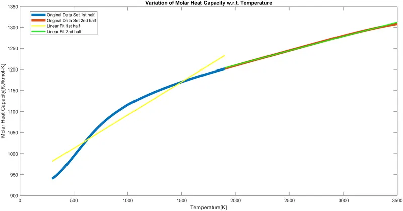
We can see that the curve fit for the 2nd half of data set is a near perfect curve fit.
- Section 3.2 -> In the second sub-section, I have written a code to calculate the S.S.E.(Sum of Squared Errors) for the obtained Linear Curve Fit(on both split data set) and the original split data set.
Attached below is my code:
%3.2
%Measuring SSE Error between curve fit(linear) and original data(Split-wise into 2 halves):
Each1SseLinSplit=0;
Each2SseLinSplit=0;
for i=1:(numel(cp_data)/4)
    Error1_SseLinSplit(i)=(cp1(i)-Predicted_CpLinSplit1(i))^2;
    Error2_SseLinSplit(i)=(cp2(i)-Predicted_CpLinSplit2(i))^2;
    Each1SseLinSplit=Each1SseLinSplit+Error1_SseLinSplit(i);
    Each2SseLinSplit=Each2SseLinSplit+Error2_SseLinSplit(i);
    Sum1SseLinSplit(i)=Each1SseLinSplit;
    Sum2SseLinSplit(i)=Each2SseLinSplit;
    SumSseLinSplit(i)=Sum1SseLinSplit(i)+Sum2SseLinSplit(i);
end
SseLinSplit=SumSseLinSplit(end);

%Plotting Sum of Squared Error(Cubic splitwise) w.r.t. Temperature:
figure(10);
plot(temperature1,Error1_SseLinSplit,'linewidth',3)
hold on
plot(temperature2,Error2_SseLinSplit,'linewidth',3)
xlabel('Temperature')
ylabel('Squared Error(calculated for Linear Fit on Split Data)')
title('Variation of Squared Error(calculated for Linear fit on split data) w.r.t. Temperature')
legend('Squared Error of 1st half of data set','Squared Error of 2nd half of data set')
The Variable SseLinSplit will store the value of S.S.E. for the obtained the net Cubic Curve Fit and the original split data set.
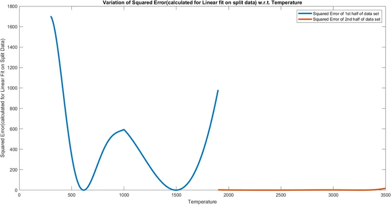
In the above code I have also given commands to plot the variation of ‘Squared Error’ (not sum) for each data point w.r.t. to the corresponding value of Temperature. The plot box has been named as Figure 10.
Attached below is the plot:
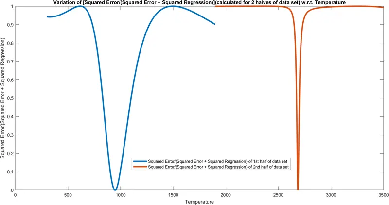
- Section 3.3 -> In the third sub-section, I have written a code to calculate the R_squared value for the obtained Linear Curve Fit(on both split data set) and the original data set.
Attached below is the code:
%3.3
%Measuring R-squared Error between curve fit(linear) and original data(split into 2 halves):
Each1_SsrLinSplit=0;
Each2_SsrLinSplit=0;
am1=sum(cp1)/numel(temperature1);
am2=sum(cp2)/numel(temperature2);
for i=1:(numel(cp1))
    Error1_SsrLinSplit(i)=(cp1(i)-am1)^2;
    Error2_SsrLinSplit(i)=(cp2(i)-am2)^2;
    Each1_SsrLinSplit=Each1_SsrLinSplit+Error1_SsrLinSplit(i);
    Each2_SsrLinSplit=Each2_SsrLinSplit+Error2_SsrLinSplit(i);
    Sum1SsrLinSplit(i)=Each1_SsrLinSplit;
    Sum2SsrLinSplit(i)=Each2_SsrLinSplit;
    SumSsrLinSplit(i)=Sum1SsrLinSplit(i)+Sum2SsrLinSplit(i);
    Each1_R_squareLinSplit(i)=Error1_SsrLinSplit(i)/(Error1_SseLinSplit(i)+Error1_SsrLinSplit(i));
    Each2_R_squareLinSplit(i)=Error2_SsrLinSplit(i)/(Error2_SseLinSplit(i)+Error2_SsrLinSplit(i));
    Sum1_R_squareLinSplit(i)=Sum1SsrLinSplit(i)/(Sum1SsrLinSplit(i)+Sum1SseLinSplit(i));
    Sum2_R_squareLinSplit(i)=Sum2SsrLinSplit(i)/(Sum2SsrLinSplit(i)+Sum2SseLinSplit(i));
    Sum_R_squareLinSplit(i)=SumSsrLinSplit(i)/(SumSsrLinSplit(i)+SumSseLinSplit(i));
end
R_squareLinSplit=Sum_R_squareLinSplit(end);

%Plotting R-squared Error(Cubic Splitwise) w.r.t. Temperature:
figure(11);
plot(temperature1,Each1_R_squareLinSplit,'linewidth',3)
hold on
plot(temperature2,Each2_R_squareLinSplit,'linewidth',3)
xlabel('Temperature')
ylabel('Squared Error/(Squared Error + Squared Regression)')
title('Variation of [Squared Error/(Squared Error + Squared Regression)](calculated for 2 halves of data set) w.r.t. Temperature')
legend('Squared Error/(Squared Error + Squared Regression) of 1st half of data set','Squared Error/(Squared Error + Squared Regression) of 2nd half of data set')
The Variable R_squareLinSplit will store the value of R-squared for the obtained Linear Curve Fit(on both split data set) and the original split data set. In the above code I have also given commands to plot the variation of for each data point w.r.t. to the corresponding value of Temperature. The plot box has been named as Figure 11.
Attached below is the plot:
- Section 3.4 -> In the 4th sub-section, I have written a code to calculate the R.M.S.E. (Root Mean Square Error) for the obtained Linear curve fit(on both split data set) and the original data points.
Attached below is the code:
%3.4
%Measuring Root Mean Square Error between data points & Curve fit(Linear(whole)):
for i=1:(numel(cp1))
    Each1_RmseLinSplit(i)=sqrt(Error1_SseLinSplit(i)/i);
    Each2_RmseLinSplit(i)=sqrt(Error2_SseLinSplit(i)/i);
    Sum1_RmseLinSplit(i)=sqrt(Sum1SseLinSplit(i)/i);
    Sum2_RmseLinSplit(i)=sqrt(Sum2SseLinSplit(i)/i);
    Sum_RmseLinSplit(i)=sqrt((Sum1SseLinSplit(i)+Sum2SseLinSplit(i))/(i+i));
end
RMSELinSplit=Sum_RmseLinSplit(end);


%Plotting Root Mean Squared Error(Cubic(split)) w.r.t. Temperature:
figure(12)
plot(temperature1,Sum1_RmseLinSplit,'Linewidth',3)
hold on
plot(temperature2,Sum2_RmseLinSplit,'Linewidth',3)
xlabel('Temperature')
ylabel('Root Mean Square Error')
title('Variation of R.M.S.E.(calculated for Linear Fit on split data) w.r.t. Temperature')
legend('RMSE of 1st half of data set','RMSE of 2nd half of data set')
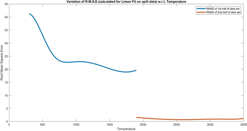
The variable RMSELinSplit will store the value of R.M.S.E. for the obtained curve fit(on both split data set) and the original split data set. In the above code, I have also given commands to plot the variation of R.M.S.E. for each data point w.r.t. to the corresponding value of temperature. The plot box has been named as Figure 12. Attached below is the plot
- Section 4 -> For this case, I have split my data into 2 equal halves This is my code to curve fit both the split data using cubic fit on the both the data and also plot the curve fit along with the raw data points. I will also determine the goodness of both the curve fits (applied curve fit separately on each half) by calculating the S.S.E. ,R-squared and the RSME values for this fit on the original data points.
- Section 4.1 -> In this sub-section, the code is written to curve fit the original data using cubic fit on each split data set and plot both curve fits along with the original data points.
My code:
%4.1
%Plot Molar Heat Capacity vs Temperature(Splitwise 2 halves for Cubic Fit):
figure(13)
plot(temperature1,cp1,'linewidth',5)
hold on
plot(temperature2,cp2,'linewidth',5)
xlabel('Temperature[K]')
ylabel('Molar Heat Capacity[KJ/kmol-K]')

%Cubic Curve Fit(Split-wise into 2 halves):
%c_p=(a*T^3)+(b*T^2)+(c*T)+d
CubeSplitCo_effs1=polyfit(temperature1,cp1,3);
CubeSplitCo_effs2=polyfit(temperature2,cp2,3);
Predicted_CpCubeSplit1=polyval(CubeSplitCo_effs1,temperature1);
Predicted_CpCubeSplit2=polyval(CubeSplitCo_effs2,temperature2);

%Compare my curve fit(cubic(spit into 2 halves)) with original data(Split-wise into 2 halves):
hold on
plot(temperature1,Predicted_CpCubeSplit1,'linewidth',2,'color','y')
plot(temperature2,Predicted_CpCubeSplit2,'linewidth',2,'color','g')
legend('Original Data Set 1st half','Original Data Set 2nd half','Cubic Fit 1st half','Cubic Fit 2nd half')
hold off
In this code I have loaded the ‘Molar heat capacity’ and ‘Temperature’ values and written a code for 3rd order polynomial fit for each (Molar Heat Capacity-Temperature) split data set using the commands ‘polyfit’ and ‘polyval’.
Then I have plotted the obtained curve fits on the curve (formed by joining the original split data set) where we can visually analyse the goodness of curve fit. The plot box has been named as Figure 13. Attached below is the plot:
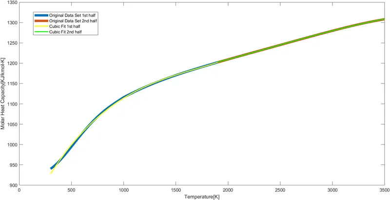
We can see that the curve fit on the the 2nd half of data set is a perfect fit.
- Section 4.2 -> In the second sub-section, I have written a code to calculate the S.S.E.(Sum of Squared Errors) for the obtained Cubic Curve Fit(on both split data set) and the original split data set.
Attached below is my code:
%4.2
%Measuring SSE Error between curve fit(cubic) and original data(Split-wise into 2 halves):
Each1SseCubeSplit=0;
Each2SseCubeSplit=0;
for i=1:(numel(cp_data)/4)
    Error1_SseCubeSplit(i)=(cp1(i)-Predicted_CpCubeSplit1(i))^2;
    Error2_SseCubeSplit(i)=(cp2(i)-Predicted_CpCubeSplit2(i))^2;
    Each1SseCubeSplit=Each1SseCubeSplit+Error1_SseCubeSplit(i);
    Each2SseCubeSplit=Each2SseCubeSplit+Error2_SseCubeSplit(i);
    Sum1SseCubeSplit(i)=Each1SseCubeSplit;
    Sum2SseCubeSplit(i)=Each2SseCubeSplit;
    SumSseCubeSplit(i)=Sum1SseCubeSplit(i)+Sum2SseCubeSplit(i);
end
SseCubeSplit=SumSseCubeSplit(end);

%Plotting Sum of Squared Error(Cubic splitwise) w.r.t. Temperature:
figure(14);
plot(temperature1,Error1_SseCubeSplit,'linewidth',3)
hold on
plot(temperature2,Error2_SseCubeSplit,'linewidth',3)
xlabel('Temperature')
ylabel('Squared Error(calculated for Cubic Fit on Split Data)')
title('Variation of Squared Error(calculated for Cubic Regression on split data) w.r.t. Temperature')
legend('Squared Error of 1st half of data set','Squared Error of 2nd half of data set')
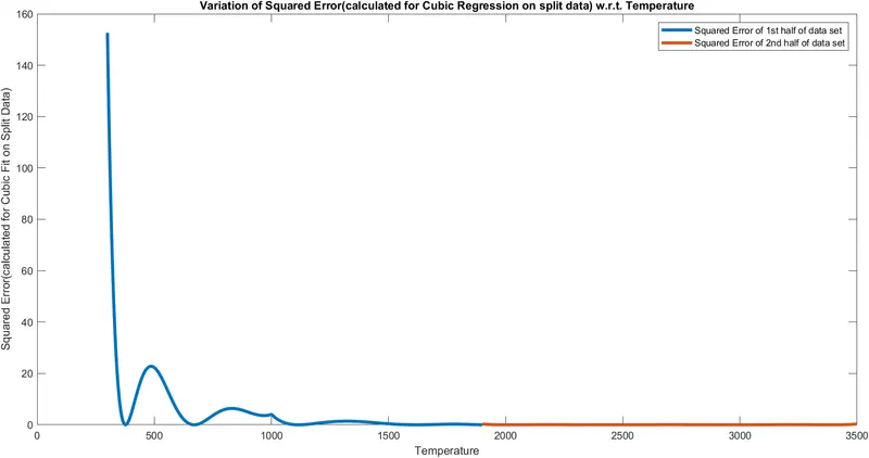
The Variable SseCubeSplit will store the value of S.S.E. for the obtained the net Cubic Curve Fit and the original split data set.
In the above code I have also given commands to plot the variation of ‘Squared Error’ (not sum) for each data point w.r.t. to the corresponding value of Temperature. The plot box has been named as Figure 14.
Attached below is the plot:
- Section 4.3 -> In the third sub-section, I have written a code to calculate the R_squared value for the obtained cubic Curve Fit(on both split data set) and the original split data set.
Attached below is the code:
%4.3
%Measuring R-squared Error between curve fit(cubic) and original data(split into 2 halves):
Each1_SsrCubeSplit=0;
Each2_SsrCubeSplit=0;
am1=sum(cp1)/numel(temperature1);
am2=sum(cp2)/numel(temperature2);
for i=1:(numel(cp1))
    Error1_SsrCubeSplit(i)=(cp1(i)-am1)^2;
    Error2_SsrCubeSplit(i)=(cp2(i)-am2)^2;
    Each1_SsrCubeSplit=Each1_SsrCubeSplit+Error1_SsrCubeSplit(i);
    Each2_SsrCubeSplit=Each2_SsrCubeSplit+Error2_SsrCubeSplit(i);
    Sum1SsrCubeSplit(i)=Each1_SsrCubeSplit;
    Sum2SsrCubeSplit(i)=Each2_SsrCubeSplit;
    SumSsrCubeSplit(i)=Sum1SsrCubeSplit(i)+Sum2SsrCubeSplit(i);
    Each1_R_squareCubeSplit(i)=Error1_SsrCubeSplit(i)/(Error1_SseCubeSplit(i)+Error1_SsrCubeSplit(i));
    Each2_R_squareCubeSplit(i)=Error2_SsrCubeSplit(i)/(Error2_SseCubeSplit(i)+Error2_SsrCubeSplit(i));
    Sum1_R_squareCubeSplit(i)=Sum1SsrCubeSplit(i)/(Sum1SsrCubeSplit(i)+Sum1SseCubeSplit(i));
    Sum2_R_squareCubeSplit(i)=Sum2SsrCubeSplit(i)/(Sum2SsrCubeSplit(i)+Sum2SseCubeSplit(i));
    Sum_R_squareCubeSplit(i)=SumSsrCubeSplit(i)/(SumSsrCubeSplit(i)+SumSseCubeSplit(i));
end
R_squareCubeSplit=Sum_R_squareCubeSplit(end);

%Plotting R-squared Error(Cubic Splitwise) w.r.t. Temperature:
figure(15);
plot(temperature1,Each1_R_squareCubeSplit,'linewidth',3)
hold on
plot(temperature2,Each2_R_squareCubeSplit,'linewidth',3)
xlabel('Temperature')
ylabel('Squared Error/(Squared Error + Squared Regression)')
title('Variation of [Squared Error/(Squared Error + Squared Regression)](calculated for 2 halves of data set) w.r.t. Temperature')
legend('Squared Error/(Squared Error + Squared Regression) of 1st half of data set','Squared Error/(Squared Error + Squared Regression) of 2nd half of data set')
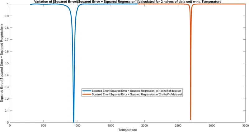
The Variable R_squareCubeSplit will store the value of net R-squared for the obtained cubic Curve Fit(on both split data set) and the original split data set. In the above code I have also given commands to plot the variation of for each data point w.r.t. to the corresponding value of Temperature. The plot box has been named as Figure 15.
Attached below is the plot:
- Section 4.4 -> In the 4th sub-section, I have written a code to calculate the R.M.S.E. (Root Mean Square Error) for the obtained cubic curve fit(on both split data set) and the original data points.
Attached below is the code:
%4.4
%Measuring Root Mean Square Error between data points & Curve fit(Linear(whole)):
for i=1:(numel(cp1))
    Each1_RmseCubeSplit(i)=sqrt(Error1_SseCubeSplit(i)/i);
    Each2_RmseCubeSplit(i)=sqrt(Error2_SseCubeSplit(i)/i);
    Sum1_RmseCubeSplit(i)=sqrt(Sum1SseCubeSplit(i)/i);
    Sum2_RmseCubeSplit(i)=sqrt(Sum2SseCubeSplit(i)/i);
    Sum_RmseCubeSplit(i)=sqrt((Sum1SseCubeSplit(i)+Sum2SseCubeSplit(i))/(i+i));
end
RMSECubeSplit=Sum_RmseCubeSplit(end);


%Plotting Root Mean Squared Error(Cubic(split)) w.r.t. Temperature:
figure(16)
plot(temperature1,Sum1_RmseCubeSplit,'Linewidth',3)
hold on
plot(temperature2,Sum2_RmseCubeSplit,'Linewidth',3)
xlabel('Temperature')
ylabel('Root Mean Square Error')
title('Variation of R.M.S.E.(calculated for Cubic Fit on split data) w.r.t. Temperature')
legend('RMSE of 1st half of data set','RMSE of 2nd half of data set')
The variable RMSECubeSplit will store the value of R.M.S.E. for the obtained curve fit(on both split data set) and the original split data set. In the above code, I have also given commands to plot the variation of R.M.S.E. for each data point w.r.t. to the corresponding value of temperature. The plot box has been named as Figure 16. Attached below is the plot:
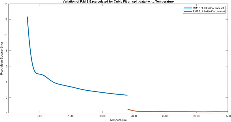
OBSERVATIONS & RESULTS:
- Along with the visual representation of the goodness of the fits, the results of the parameters (like R-squared, SSE and R.S.M.E.) also give a strong conclusion on the fitness characteristics of the curve.
- The results obtained are as follows:
|
Fit Type |
Parameter results from my code output |
Parameter results found by using Curve Fitting Tool of MATLAB |
|
1st order(Linear) polynomial fit on whole data set |
Sum of Squares of Error (S.S.E.) = 2.1630 x 10⁶ |
Sum of Squares of Error (S.S.E.) = 2.1630 x 10⁶ |
|
1st order(Linear) polynomial fit on whole data set |
R-squared value=0.9301 |
R-squared value=0.9249 |
|
1st order(Linear) polynomial fit on whole data set |
Root Mean Square Error(R.M.S.E.)=25.9991 |
Root Mean Square Error(R.M.S.E.)=26.0072 |
|
3rd order(Cubic) polynomial fit on whole data set |
Sum of Squares of Error (S.S.E.)=9.4272 x 10⁴ |
Sum of Squares of Error(S.S.E.)=9.4272 X 10⁴ |
|
3rd order(Cubic) polynomial fit on whole data set |
R-squared value=0.9967 |
R-squared value=0.9967 |
|
3rd order(Cubic) polynomial fit on whole data set |
Root Mean Square Error(R.S.M.E.)=5.4277 |
Root Mean Square Error(R.M.S.E.)=5.4311 |
|
1st order polynomial fit done separately on 2 equal halves of original data set |
Net Sum of Squares of Error (S.S.E.) = 6.1949 X 10⁵ |
Sum of Squares of Error 1(S.S.E.1)=6.1721 X 10⁵ Sum Of Squares of Error 2(S.S.E.2)=2.2842 X 10³ Net Sum of Squares of Error(S.S.E.)=S.S.E.1 + S.S.E.2 = 6.194942 x 10⁵ |
|
1st order polynomial fit done separately on 2 equal halves of original data set |
Net R-squared value = 0.9451 |
R-squared 1(R12)= 0.9320 R-squared 2(R22) = 0.9986 Net R-squared value = = 0.9322 |
|
1st order polynomial fit done separately on 2 equal halves of original data set |
Net Root Mean Square Error (R.M.S.E.)= 13.9137 |
Root Mean Square Error 1(R.M.S.E.1)=19.6529 Root Mean Square Error 2(R.M.S.E.2)=1.1956 Net Root Mean Square Error (R.M.S.E.net)= =13.9225 |
|
3rd order polynomial fit done separately on 2 equal halves of original data set |
Net Sum of Squares of Error (S.S.E.) = 8.4871 x 10³ |
Sum of Squares of Error 3(S.S.E.3)=8.4353 X 10³ Sum Of Squares of Error 4(S.S.E.4)=51.8019 Net Sum of Squares of Error(S.S.E.)=S.S.E.3 + S.S.E.4 = 8.4871019 X 10³ |
|
3rd order polynomial fit done separately on 2 equal halves of original data set |
Net R-squared value = 0.9992 |
R-squared 3(R32)= 0.9991 R-squared 4(R42) = 1.0000 Net R-squared value= = 0.9991054 |
|
3rd order polynomial fit done separately on 2 equal halves of original data set |
Net Root Mean Square Error=1.6286 |
Root Mean Square Error 3(R.M.S.E.3)=2.2990 Root Mean Square Error 4(R.M.S.E.4)=0.1802 Net Root Mean Square Error (R.M.S.E.net) = = 1.6307 |
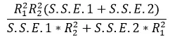

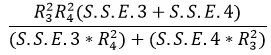

In the above table, the terms:
- S.S.E.1 -> Sum of Squares of Error calculated for linear polynomial fit on 1st half of data set.
- S.S.E.2 -> Sum of Squares of Error calculated for linear polynomial fit on 2nd half of data set.
- S.S.E.3 -> Sum of Squares of Error calculated for cubic polynomial fit on 1st half of data set.
- S.S.E.4 -> Sum of Squares of Error calculated for linear polynomial fit on 2nd half of data set.
- R12 -> R-squared value calculated for linear polynomial fit on 1st half of data set.
- R22 -> R-squared value calculated for linear polynomial fit on 2nd half of data set.
- R32 -> R-squared value calculated for cubic polynomial fit on 1st half of data set.
- R42 -> R-squared value calculated for cubic polynomial fit on 1st half of data set.
- R.M.S.E.1 -> Root Mean Square Error calculated for linear polynomial fit on 1st half of data set.
- R.M.S.E.2 -> Root Mean Square Error calculated for linear polynomial fit on 2nd half of data set.
- R.M.S.E.3 -> Root Mean Square Error calculated for cubic polynomial fit on 1st half of data set.
- R.M.S.E.4 -> Root Mean Square Error calculated for cubic polynomial fit on 1st half of data set.
CONCLUSION:
- From the analysis of the plots as well as the results of the parameters(describing the goodness of the curve fit),we can conclude that:
- The goodness/quality of the curve fit increases as we increase the order of the polynomial equation to best fit the original data points. This is evident as the cubic curve fit better fits the data points than the linear fit.
- If I want to improve the quality/goodness of the curve fit keeping the order of the polynomial equation used for curve fit intact, then the goodness of the curve fit can be increased by splitting the data points into parts and then applying curve fit for each part. This method of fitting the curve fit is known as split wise method of fitting the curve and as evident from the results, the goodness of curve fit increased after splitting the original data and then applying the curve fit on each part.
- MATLAB is an excellent means to apply curve fit via various techniques on a given data set.
ANSWERS TO SOME IMPORTANT QUESTIONS:
- How to make a curve fit perfectly?
Ans: This can be answered by analysing the number of bends as one progresses over the sequence of the co-ordinates of the given data set (Molar Heat Capacity-Temperature).Each increase in the exponent(order of the polynomial equation) produces one more bend in the curve fitted line. This can be done by joining all the data points and counting the number of bends of the curve formed by joining the data points. The order of the polynomial equation to be used for curve fitting the original data set can be set equal to the total number of bends of the curve (formed by original data set) in order to make the curve fit perfectly. Perfect fit is a fit in which all the co-ordinates of the original data set fall within the curve fit.
For example, in my project, the cubic fit applied on the 2nd half of the data set fits all the data points perfectly. This can be visually verified from the curve fit plot as well as analytically where we can see that the R-squared value for this curve fit has come out as 1.00(the best possible R-squared value for a curve fit) which indicates that this curve fit fits the 2nd half of the data set perfectly.
- How to get the best fit?
Ans: The answer to this question can be linked to the conclusions drawn from this project. As can be seen from the results, we can say that the goodness of the fit increases as we increase the order of the polynomial equation used for fitting the original data set. The best possible fit is the curve fit that encompasses maximum possible data points. Even after getting the required order of the polynomial equation that will be used as a curve fit we can split the original data set into appropriate parts and see to what extent the curve fit manages to encompass the data points than it managed to encompass the when the curve fit was applied to the entire data set at once.
Applying the above ways in a trial & error fashion will enable us to get the best fit for the curve (formed by original data set).The best fit may or may not be the perfect fit for the curve(formed by original data set).
- What could be done to improve cubic fit?
Ans: As I had explained in the Conclusions section, the improvement in goodness of any given order of a polynomial fit (not just cubic fit) can be done by splitting up the given data set into parts and then applying the required order of polynomial fit on each part (for case mentioned in the question, it will be applying cubic fit on each part).
ERRORS FACED WHILE PROGRAMMING:
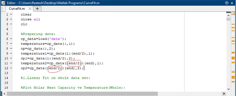
- Misjudgement in assigning the range of loaded data set to variables for implementing the split wise method of curve fitting:
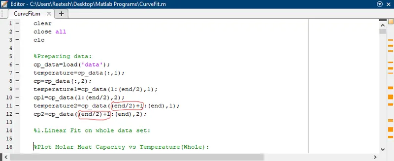
While assigning the range of data set to separate variables (dependent & independent) needed to implement the split-wise method of curve fit, I had initialised two sets of variables (independent & dependent) where each set takes gets an equal half of the original data set. In the original data set, there are 3200 values of Molar heat capacity corresponding to 3200 values of temperature. While splitting the data set into 2 equal halves, I wanted to assign 1st 1600 values of Molar heat capacity to variable cp1 and the last 1600 values of Molar Heat capacity to variable cp2.Similarly I wanted to assign 1st 1600 values of temperature to variable temperature1 and the last 1600 values of Temperature to variable temperature2. But while assigning the range of data set to the variables, I assigned the range of 1st half of data set from 1st element to the element in the 1600th position and the range of 2nd half of data set also from 1600th element to 3200th element. Firstly, these parts of data set are not equal as the 1st half has 1600 elements while the 2nd half of data set has 1601 elements. The last element in the in the 1st half of data set is again included as the 1st element in the 2nd half of data set.
Mistake made:
Output due to mistake:

Correction made:
- Mistake 2: Not saving the .m program file in the same folder as that of the file containing the original data.
Output due to this mistake: The code will not run and this error message will be displayed:
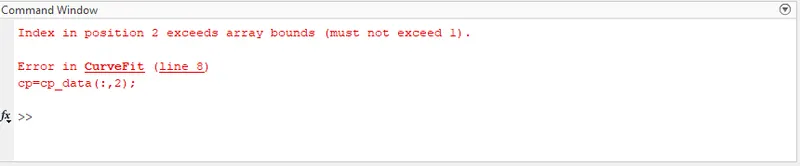
Correction made: Saved the program file (.m extension) in the same folder as that of the file containing the original data.
REFERENCES: