SoC Estimation of a Battery Pack

OBJECTIVES:

https://in.mathworks.com/matlabcentral/fileexchange/72865-design-and-test-lithium-ion-battery-management-algorithms

Download the Files from the above Link, open the Project in MATLAB and do the following:

1. Simulate the 3 test cases from Harness Dashboard and write a detailed report on the results.
2. What is coulomb counting? Refer to the above model and explain how BMS implements coulomb counting for SOC estimation?

SOLUTIONS:

Solution to Objective 1:

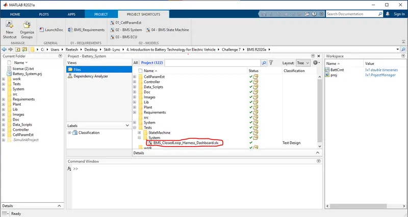
The Project is loaded in MATLAB by navigating to the Folder in the ‘Current Folder’ Section where the original Project File is kept.

The Project File (File Name: Battery_System.prj) is loaded into MATLAB by double-clicking on it.

Once everything has been loaded, under the Project Section, extend the ‘Tests’ Folder, then again extend the ‘System’ Folder and double click on ‘BMS_ClosedLoop_Harness_Dashboard.slx’ Simulink File:

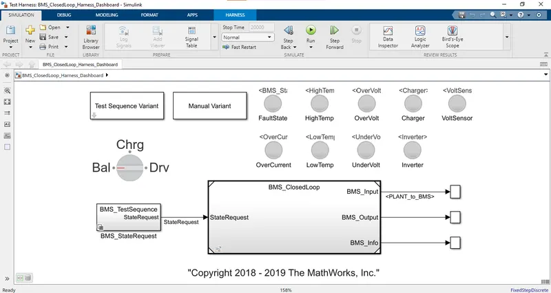
The Closed Loop Harness Dashboard Simulink Model containing various subsystems:

Test Case 1:

The ‘Test Sequence Variant’ Subsystem is double-clicked and the Test Case ’1’ is chosen:

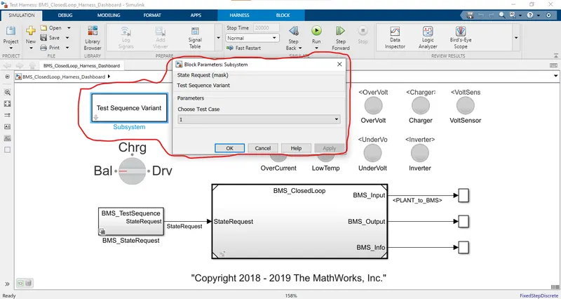
There is no way to change the Simulation Time. The ‘Run’ Button is now pressed to run the Simulation of the Model for Test case 1.

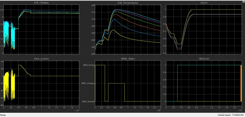
According to the Simulation Results, the following can be commented on the results of Various Parameters of the Cell(s)/Module(s):

SOC:

• The SOC is initially for the Cell(s) is set to 0.8 or 80% and the SOC is calculated using the method of Coulomb Counting (Yellow Curve), E.K.F. (Extended Kalman Filter) (Orange/Red Curve) & U.K.F. (Unscented Kalman Filter) (Blue Curve).
• The SOC of the Cells for all the 3 curves keep decreasing as the Pack Current Extracted from all the Battery Pack and delivered to the Load remains positive (above 0) and correspondingly the SOC of the Cell(s) increases as the Pack Current becomes negative (Pack Current is now distributed to the Cell(s) hence increasing their capacity).
• The SOC of the Cell(s) remains constant as long as the Pack Current becomes 0 (i.e. no Current is flowing from/into the Cell(s)).
• From my analysis of Behaviour of the 3 SOC Measurement Techniques, the SOC Measurement Technique displayed by the Yellow Curve looks very ideal and is matching in every aspect to the corresponding behaviour of the Pack Current.
• The SOC Measurement displayed by the other 2 curves (Blue & Red Curves), seem more realistic because in real case scenarios, if 2 parameters are related, then change and behaviour of 1 of the parameters doesn’t correspondingly bring about a change in the other parameter as per the defined relation because in real case scenarios a lot of other factors are to be taken into consideration which are not generally taken into consideration in ideal case scenarios. Hence the 2 curves seem to display a more realistic SOC behavioural pattern w.r.t. to the Pack Current curve with the Red Curve displaying a slightly more realistic scenario as more the reality there is in the real case scenarios, more will be the losses involved in System working as seen in practical cases.

Cell Voltages:

• The Cell Voltages are initially set to 3.85 V to 3.9 Volts.
• The Cell Voltage(s) Behaviour resonates behaviour of the Pack Current which indicates that the Cell(s) are able to dispatch/receive energy as per the Load Demands (Pack Current). However all this was while the BMS was at Standby State.

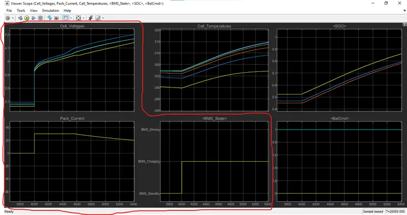
• At around 4000 seconds, when the Pack Current suddenly rises upto 30 Units leading to an equivalent rise in the Cell Voltage(s), the BMS moves from ‘Standby State’ to ‘Charging State’, and then Pack Current then remains constant till about 4560 seconds, but the Cell Voltages still increased during this Constant Current Period but after 4560 seconds, a significant decrease in Pack Current in order to reduce the limit the Cell Voltage (which had gone upto 4.2 V by then) is successful and the Cell Voltage remains constant during this time frame until at around 7152 seconds, the Pack Current suddenly drops from 3 Amperes to 0 Amperes and the Cell Voltage also undergo a similar drop after which all the Cell Voltage(s) are seen tending to converge.

Cell Temperatures:

• Initially all the Cell Temperatures were at a similar value(at the start of simulation), however as the time period for which Current Activity in the Cells increased, the Cell Temperatures kept on increasing and each Cell Temperature increased more rapidly and steeply than the other with Cell 6 exhibiting the highest Temperature.
• As the Pack Current suddenly increased at 4000 seconds, the Cell Temperature(s) also showed an exponential increase, with Cell 6 exhibiting the steepest increase and Cell 1 exhibiting the lowest increase.
• Each Cell temperature Behaviour during the Pack Current’s Sudden increase at 4000 seconds: Cell 1 Temperature < Cell 2 Temperature < Cell 3 Temperature < Cell 4 Temperature < Cell 5 Temperature <= Cell 6 Temperature.

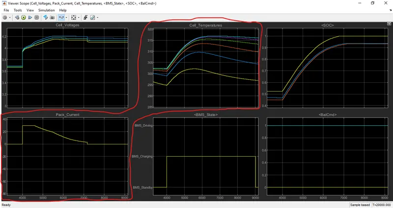
• However when the Pack Current becomes 0 at around 7000 seconds, the Cell Temperatures start decreasing steadily till the end of Simulation Time where the Final Cell Temperature(s) State for Each Cell are: Cell 1 Temperature < Cell 2 Temperature < Cell 3 Temperature < Cell 4 Temperature < Cell 5 Temperature < Cell 6 Temperature.

Pack Current:

• The Pack Current variation is similar to the Cell Voltage(s) variation when the BMS is at Standby Mode.
• However when the Pack Current suddenly increases from 0 to 30 Units, the BMS changes from Standby State to Charging State which ensures that the Cell Voltage(s) stay within the Limit by first ensuring that their increase rate is decreased and then their Variation becomes constant. In order to ensure that the Cell Voltage(s) variation becomes constant and within Limits, the Pack Current is subsequently decreased.

BMS State:

• The BMS keeps the Battery Stack in Driving State as long as there is an overall Positive Current in the Pack Current Plot i.e. the Cells are overall discharging Current to the Load. At around at 3000 seconds, the BMS goes to a Standby State on account of Pack Current becoming 0.
• At around 4000 seconds, the Pack Current suddenly rises from 0 to 30 which tends to push the Cell Voltage(s) beyond its threshold limit. Hence the BMS steps in from ‘Standby’ State to ‘Charging’ State to prevent the further rise in Current and to stop the Cell Voltage(s) from crossing its own threshold limit.
• When The BMS state comes to ‘Charging State’, the Pack Current stays constant at 30, but still the Cell Voltage(s) continue to increase, however the Cell Voltage doesn’t go beyond its threshold limit and from that threshold, either stays constant or decreases at a very very slow rate which causes the Pack Current to then decrease.
• The BMS stays at Driving State until the Pack Current substantially reduces to 0 and remains 0 and the Cell Voltage(s) stabilises within their threshold limit and then the BMS State returns to ‘Standby’ State.

Balance Command (BalCmd):

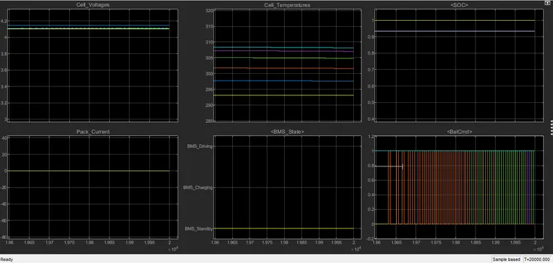
• Initially the Balance Command stays at 0 till 3000 but after that, the Cell Balance Commands gets activated (reaches value 1) for all the cells except in Cell 1.

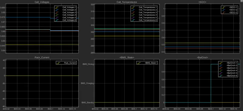
• This indicates that the Cell Balancing starts for all the cells except for Cell 1 w.r.t. Cell 1.
• At the end of simulation, the Cell Balance frequently interchanges between 0 and 1 for all the Cells except Cell 1(Yellow Curve) and Cell 6.
• Cell 1 Balance Command never gets activated (value never shifts to 1).
• Cell 6 Balance Command, once after it got activated at 3000 seconds, never dropped to 0 till the end of Simulation Time.
• Due to the activation of all the Cell Balance Commands except for Cell 1, we can see that all the Cell Voltages steadily converge once the Pact Current has reached 0 permanently.

Test Case 2:

The ‘Test Sequence Variant’ Subsystem is double-clicked and the Test Case ’2’ is chosen:

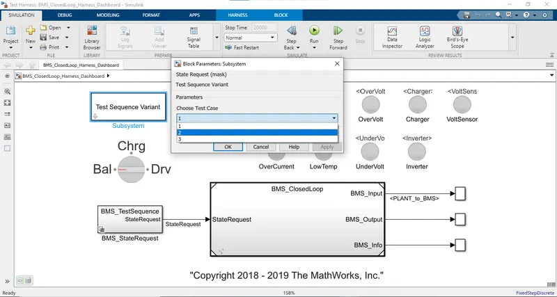
There is no way to change the Simulation Time. The ‘Run’ Button is now pressed to run the Simulation of the Model for Test case 2.

According to the Simulation Results, the following can be commented on the results of Various Parameters of the Cell(s)/Module(s):

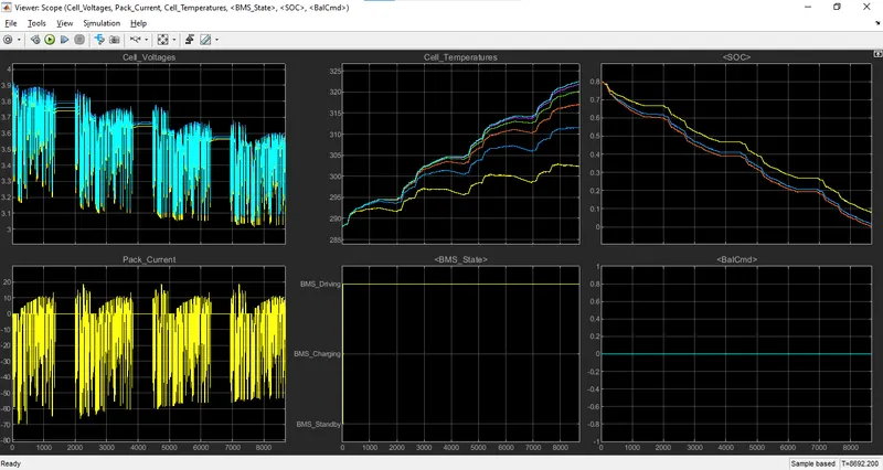
On general Observation, the Simulation Time is set to 20000 seconds, but the Simulation terminates only at 8692.200 seconds.

Pack Current:

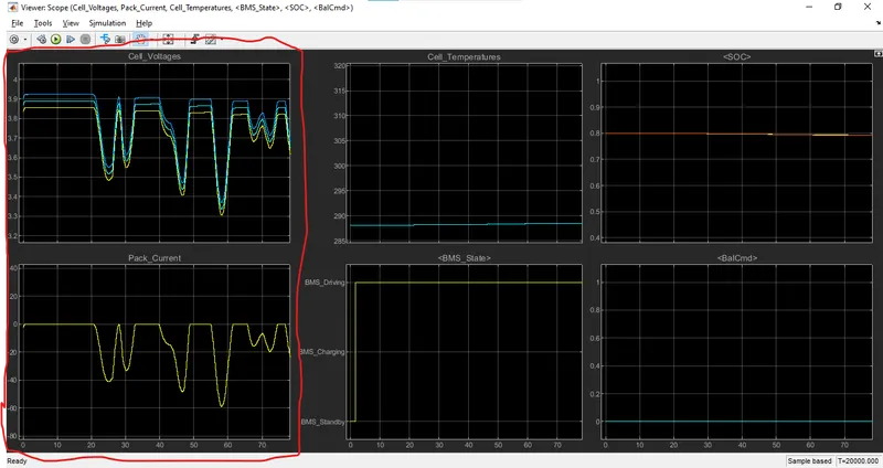
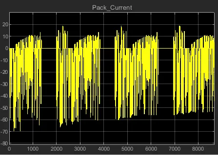
• The Drive Cycle is very demanding as is evident from the profile of the Pack Current. The Pack Current is very heavy which will lead to Cell Voltage depleting very quickly (unless it is sufficiently recharged) or Cell Temperatures rising quickly as there is seldom any situation of 0 Pack Current in this Test Case.
• Whenever there is an Overcurrent, the charger/Load is diconnected which leads to the Pack Current becoming 0. This detection of Overcurrent and disconnecting/connecting the Load/Charger to the Battery Pack is done by the BMS.
• When the Pack Current becomes 0,Cell Voltage(s) & Temperature of the Cell(s) will fall.
• As per the Pack Current Profile, most of the Current in the Pack Current Plot for the given Simulation Time is below 0 (negative Current).
• Most of the Current in the Pack Current Plot for the given Simulation Time being below 0 indicates that for most amount of time, the Cells are discharging Current to provide for the Load Demand, the signals of which are related to the Pack Current.
• Since the Pack Current is being negative which indicates that for most of time the Cells are discharging Current and the magnitude for negative Pack Current remains high(as high as -70 Amperes) throughout the majority of the time and the magnitude of Positive Pack Current remains very low for whatever time it is above 0. Hence for most of the time, the cells are discharging a very High amplitude of Current.

Cell Voltages:

• As seen in Test Case 1, similarly in Test Case 2, the behaviour of Cell Voltages reciprocates the profile of Pack Current.
• Since the Pack Current is negative throughout most of the time period, the Cell Voltage(s), the Cell Voltage(s) in overall will always be lesser than the initial Cell Voltage value.

Cell Temperatures:

• Thanks to the Heavy Pack Current (in accordance to the Heavy Demand from Load/Drive Cycle), it is seen that in overall, the Cell Temperatures keep on rising.
• For whatever time, the Cell Temperature(s) are constant or decreasing is because of the Pack Current becoming 0.
• In this case too, there is quite a significant difference in the Final Cell Temperature between Cell 1 and Cell 6.
• Due to Heavy Pack Current (Overall Discharging), there is a rapid rise in Cell Temperature(s) in this test case compared to Test Case 1.

BMS State:

• From the Start to the End of Simulation Time, once the Battery Stack has been connected to the Load, the BMS State moves to Driving State for the entirety of the Run Time by the model as throughout the Simulation the Pack Current is heavy with most Current Data in the Negative side (indicates Battery discharging condition).

Balance Command:

• The Balance Command remains at 0 for the entirety of the Simulation Time which suggests that none of the parameters cross their threshold values for whatever time the model has simulated.

SOC:

• The SOC indicated by the red curve(SOC Estimation Technique: E.K.F.) reaches 0 at 8692.200 seconds which indicates that the Battery Stack will not be able to discharge Current anymore hence indicating termination of Simulation Time set to 20,000 seconds.
• The SOC Curves indicated by the Blue Curve (SOC Estimation Technique: U.K.F.) and the Yellow Curve (SOC Estimation Technique: Coulomb Counting) have not yet reached 0. This means that the Simulation Terminates when at least 1 of the 3 SOC Estimation techniques reaches SOC=0. SOC=0 indicates that the Battery Capacity has reached 0.

Test Case 3:

The ‘Test Sequence Variant’ Subsystem is double-clicked and the Test Case ’3’ is chosen:

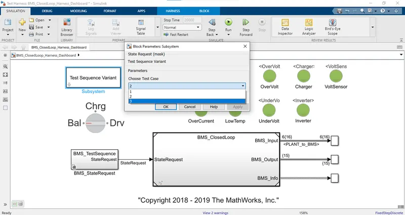
There is no way to change the Simulation Time. The ‘Run’ Button is now pressed to run the Simulation of the Model for Test Case 3.

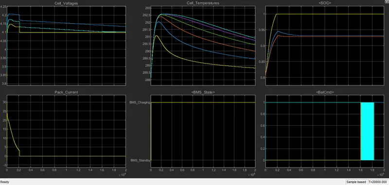
According to the Simulation Results, the following can be commented on the results of Various Parameters of the Cell(s)/Module(s):

Pack Current:

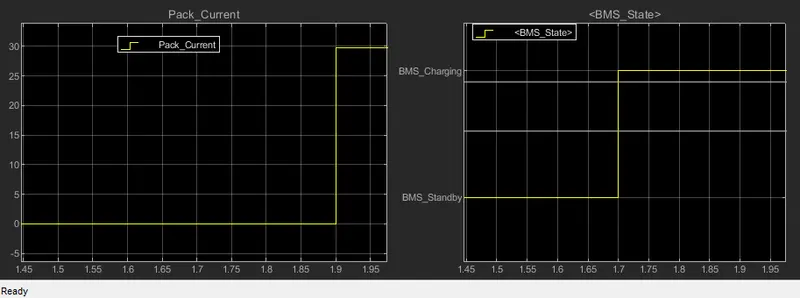
• At the initial stage, at the beginning of Simulation Time, the Pack Current was -2.322 Amperes. At nearly 1.7 seconds, the Current moved to nearly 29.8 Amperes, and later after heavy Charging Current, the Pack Current decreases to 3 Amperes at 2115.1 seconds and at 2115.1 seconds, it decreases to 0 Amperes.
• Once the Pack Current reaches 0 Ampere value, it remains at 0 Ampere Value for the rest of Simulation Time.

Cell Voltage(s):

• The Cell Voltage(s) seems to increase with decrease in Pack Current in the initial stages after the BMS State goes from ‘Standby’ State to ‘Charging’ State.

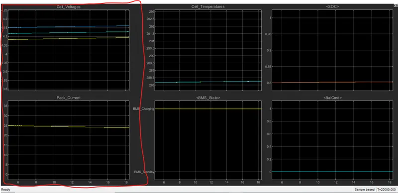
• The Cell Voltage(s) seem to vary as per the Pack Current in the initial stage but once Pack Current becomes 0, the Cell Voltage of Cell 1 becomes constant while the Cell Voltages of the other Cells of the other Cells which are on the higher side start decreasing steadily to converge with the Cell 1 Voltage as the Cell Balance Command kicks in from the very first instance itself.

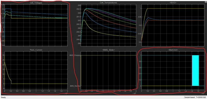
Cell Balance Command:

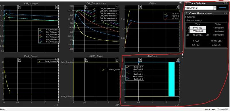
• The Cell Balance Command for all the Cells except Cell 1 kicks in at 20.1 seconds.

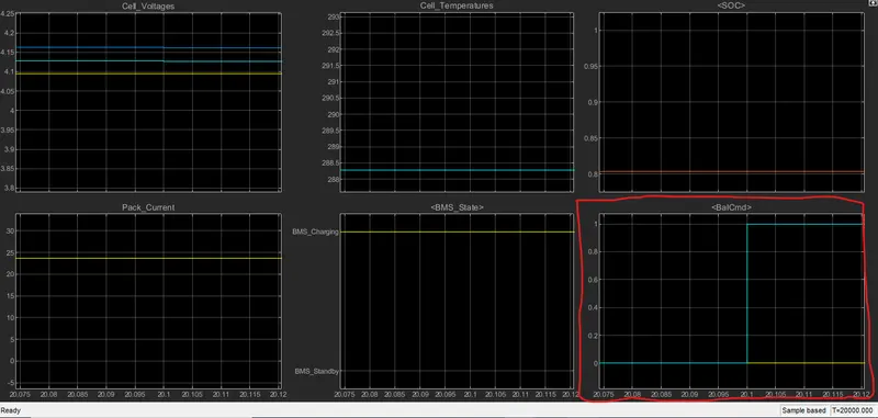
• Due to this Cell Balancing done on all the Cells except Cell 1 which causes the Cell Voltage Curves of all the Cell except Cell 1 to converge towards Cell 1 Voltage Curve.
• Nearing the end of simulation, there are frequent interchanges between Cell Balancing Commands ON & OFF for all the cells and at the end of Simulation, the Balance Command for only the Cell 2 is turned ON, while for the rest for the Cells, the Balance Command is turned OFF.

Cell Temperature(s):

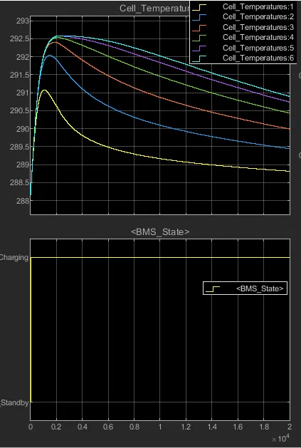
• The Cell temperatures rises sharply in response to the High Discharging & Charging Pack Current flowing in/out of the Cell(s).
• Once the Pack Current becomes 0, the Cell Temperatures slowly decreases till the end of Simulation where the Final Cell Temperature(s) State for Each Cell are: Cell 1 Temperature < Cell 2 Temperature < Cell 3 Temperature < Cell 4 Temperature < Cell 5 Temperature < Cell 6 Temperature.

BMS State:

• From Start of Simulation Time to 1.7 seconds, the BMS State remains in ‘Standby’ State and jumps to ‘Charging’ State at 1.7 seconds despite the Pack Current going from initial State of 0 Amperes to 30 Amperes in approximately 1.9 seconds and remains in this state till end of Simulation.

SOC:

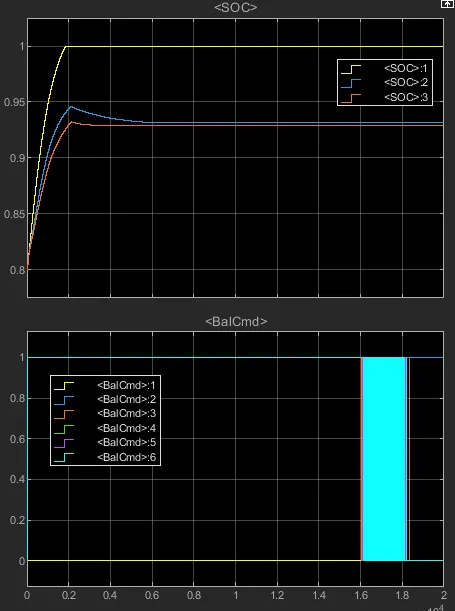
• SOC Plot has three curves which shows 3 different techniques to calculate the SOC of the Battery Pack as per the Pack Current moving in/out of the Battery Pack during simulation.
• In the SOC Plot, the Yellow Curve represents the SOC calculated by Coulomb Counting Method, Red Curve represents the SOC calculated by

E.K.F. and the Blue Curve represents the SOC calculated by U.K.F.

• The SOC calculated by Coulomb Counting reaches 100% or 1 at about 1850 seconds and stays there till the end of simulation, while the SOC estimated by U.K.F. extends to 95% (at about 2135 seconds) before slowly decreasing to 93.14%(at simulation end).
• The SOC estimated by E.K.F. extends to 93.22% (at about 2118.50 seconds) after which it slowly decreases to 92.87% (at simulation end).

Solution to Objective 2:

Coulomb Counting: It is a method to estimate the State of Charge of a Cell/Battery based on the Cell/Battery Current information and other parameters. The SOC is obtained from integration of the Cell/Battery Current using the fundamental definition of charge:

where i(t) is the time varying Current flowing in the circuit to/from the Load.

If the Initial Capacity of the Cell is known then, SOC can be obtained by dividing equation (1) with the Initial Capacity of the Cell and the SoH of the cell/Battery:

where

i(t) is the time varying Current flowing in the circuit to/from the Load.

C_p is Initial Capacity of the Battery/Cell.

SoH is the State of Health of the Battery/Cell.

This method tends to accumulate errors if it is based only on the Cell/Pack Current. Hence other parameters like Voltage of the Pack/Cell is implemented in the Battery Pack Model to implement a more observer-based SOC Estimation Method. Still it can be accurate if & only if the SoH (State of Health) & Current is precisely and accurately measured and if the initial capacity of the Battery is known.

The SOC Estimation Techniques have been implemented in the subsystem SOC_Estimation (SOC_Estimation) inside the BMS ECU (BMS_Software) subsystem which is present inside the subsystem named BMS_ClosedLoop which is present inside the main system named BMS_ClosedLoop_Harness_Dashboard.

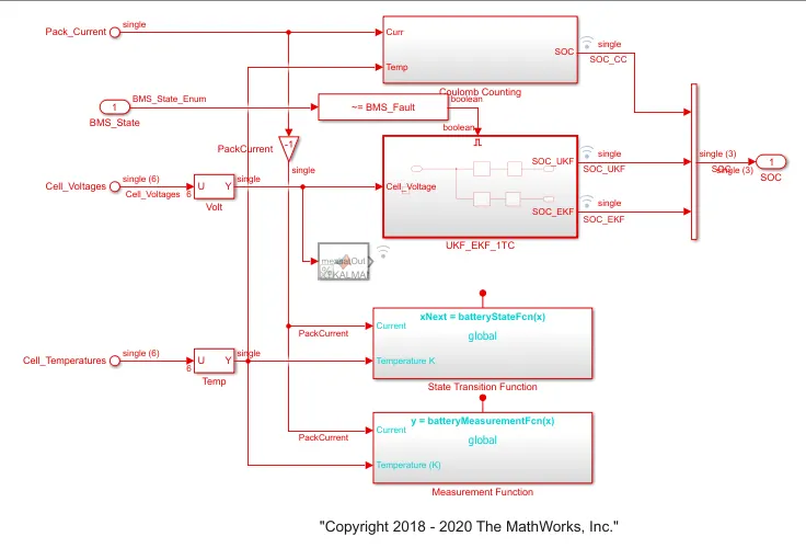
SOC Estimation Subsystem

A subsystem has been implemented in the SOC_Estimation (SOC_Estimation) named ‘Coulomb Counting’ where the SOC Estimation using the Coulomb Counting has been implemented. This subsystem takes input of the Pack Current and the Cell Temperatures for all the time instances.

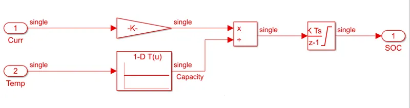
Coulomb Counting Subsystem

In the Subsystem the SOC is calculated using taking inputs of the Pack Current and the Cell Temperatures. The Cell Temperature(s) values are fed to a 1-D Lookup Table which outputs the Cell Capacity in accordance to the mapping done in the Lookup Table in response to the Cell Temperature Values fed to it.

The Pack Current input value is divided by (1/3600) in order to convert the units from Ampere into Ampere Hour.

Now the Capacity output from the 1-D Lookup Table and the Pack Current divided by (1/3600) is now fed to a ‘Divide’ Block where the Pack Current divided by (1/3600) output value is divided by the Cell Capacity output from the Lookup Table.

The output value from this ‘Divide’ Block is now fed to a Discrete Time Integrator Block where the output value from the ‘Divide Block’ is integrated discretely over Simulation Time and the SOC can be obtained for each time instance.

Given the way the SOC Estimation Method: Coulomb Counting, has been implemented in the model, the designer of this model takes into account that the SoH (State of Health) of the Cell/Battery is 1 which happens to be case for most new Batteries/Cell(s) and relies on the Measured current data and the Initial Capacity Data computed using a Lookup Table which takes Cell Temperature(s) as input, to deliver the accurate and precise SOC of the Battery Pack.