PID Controller Mathematical Modelling, Spring Mass Damper System Mathematical Modelling & Traffic Light Control Logic Modelling in Simulink

OBJECTIVES:

1. Develop a PID Controller of a second order differential equation. Equation model is given directly as a transfer function. Also, P – I – D tuning parameters are also shared to avoid spending time on tuning of controllers. Develop model using both PID Library block & also using individual gain blocks for P – I – D

Transfer Function: 20/(s^2+10s+20)

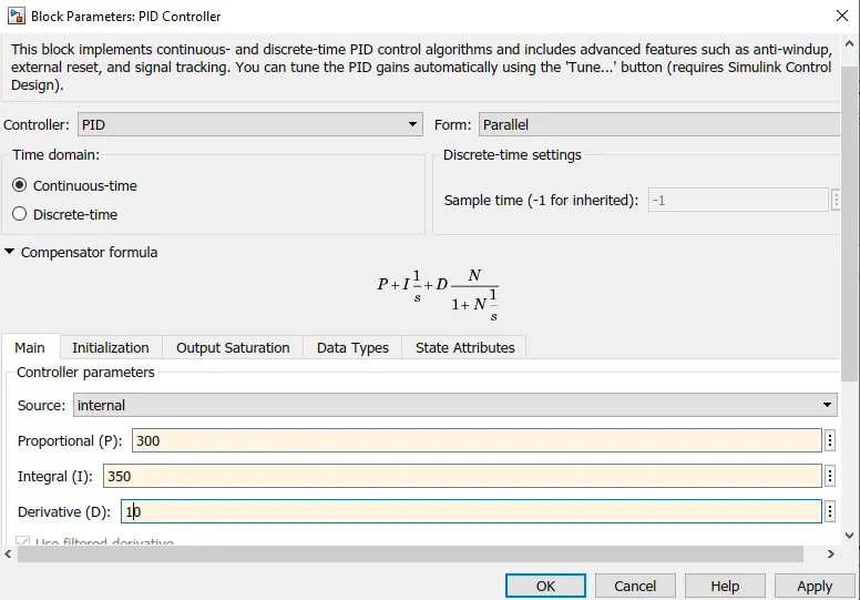
K_p=300

K_i=350

K_d=10

(Hint: https://skill-lync.com/knowledgebase/introduction-to-pid-controller-and-transfer-function)

2. To model a Spring-Mass-Damper System using Simulink. Schematic representation of Spring-Mass-Damper System:

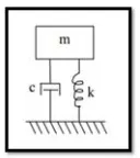
The response of the system is governed by 2^nd Order Differential Equation:

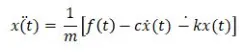
where ẍ(t) = Acceleration of the mass m.

ẋ(t) = Frequency

x(t) = Displacement

f(t) = Forcing Function

c = Damping Coefficient

k = Spring Constant

3. Create a Traffic Signal Control Logic using Stateflow charts for the following system requirement.

RED light is the default entry state (Entry value at RED state is 1 & Exit Value is 0)

YELLOW light becomes active after 5 seconds (Entry value at YELLOW state is 1 & Exit Value is 0)

GREEN light becomes active after 2 seconds (Entry value at GREEN state is 1 & Exit Value is 0)

Signal Exits GREEN state to RED state after 5 seconds.

SOLUTIONS:

Solution to Objective 1:

Theory: It is generally an instrument used in Control Applications to regulate Process Variables. This process Variables can be Temperature, Speed, Flow, etc. A PID Controller uses a Control Loop Feedback Mechanism to control these Process Variables. The Control Loop Feedback Mechanism is used to improve the accuracy and precision (as close to the Target or Setpoint) of these Output and also stabilises them.

Working Principle: In general, a PID controller combines proportional control with additional integral and derivative adjustments which help the unit automatically compensate for changes in the system.

The Transfer Function used to theoretically represent the System’s Output for the given input is as follows:

My Simulink Model to develop a PID Controller Model based on the above Transfer Function using the PID Controller Block is as follows:

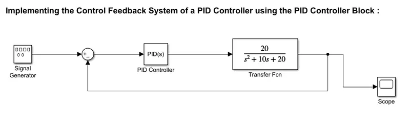
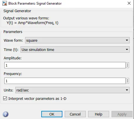
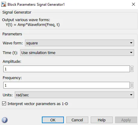
The Input to the System is generated using a Signal Generator. For this case, the Input Signal is a Square Waveform with the following parameters:

The Parameters assigned to the PID Controller Block is as follows:

My Simulink Model to develop a PID Controller Model based on the above Transfer Function using Gain & Integrator Blocks is as follows:

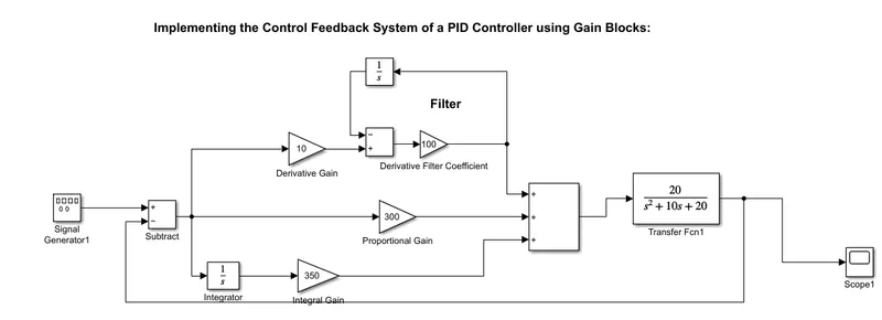
In the above model, the PID Controller has been implemented using Gain Blocks, Integrator Blocks and the Subtract Block. The Gain Blocks, Integrator Blocks and the Subtract Block have been used to implement the Output Equation of a PID Controller which is fed as an input to the Transfer Function. The actual Input is generated as a Square Wave with the following parameters:

The Output of the PID Controller takes into account the Proportional Gain (K_p) of the Output and also the Derivative and Integral of the Output (computed by the Controller) which basically represents the Error between the Desired Output (Actual Input to the System) and the Actual Output.

Result:

In the 1^st Model, where the PID Controller Block has been used to model a PID Controller, the Scope Result on running the Model is as follows:

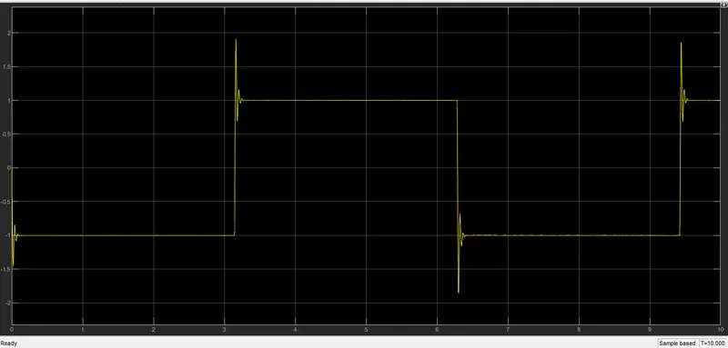
In the 2^nd Model, where Gain, Integrator and Subtract Block(s ) have been used to model a PID Controller, the Scope Result on running the Model is as follows:

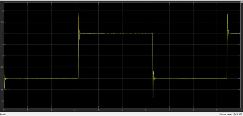
As can be seen from the Results, the Output Waveform(s) in both the cases is same.

Solution to Objective 2:

Theory: A Spring-Mass-Damper System is a system in which apart from the structure (mass m), a spring and a damper is also present. The Forces acting in a Spring-Mass-Damper System is as follows:

• Inertia Force: This Force is always acting against the change in state of the Structure (mass m), therefore it always acts against the direction of deflection of the System.
• Spring Force: This Force acts against the deflection of spring. Deflection of mass m will deflect the spring as well in that direction, so it will also act against the direction of deflection.
• Damping Force: This Force will try to damp out the Vibrations, so it will act against the deflection of spring. Hence it will also act against the direction of deflection of spring.
• Applied Force: This is the Force that is applied externally on the system and causes the system to deflect.

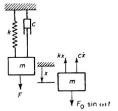
Basic Diagram & FBD of Spring-Mass-Damper System due to Forced Vibrations

Governing Equation: The Standard Equation of a Spring-Mass-Damper System for Forced Vibrations can be established using D’Alembert’s Principle. According to D’Alembert’s Principle:

All External Forces + Inertial Forces = 0

(Spring Force + Damping Force – Applied Force) + Inertia Force = 0 ______ (1)

The External Forces acting on the System are the Spring Force, the Damping Force and the Applied Force on the System.

Therefore Equation (1) can be represented by:

[-F(t) + F­_s + F_d ] + F_i = 0

where F(t) = Applied Force on the System

F­_s = Spring Force

F_d = Damping Force

F_i = Inertia Force

The Inertia Force (F_i) = mẍ

The Spring Force (F_s) = kx

The Damping Force (F_d) = cẋ

ẍ(t) = Acceleration of the mass m.

ẋ(t) = Frequency

x(t) = Displacement

f(t) = Forcing Function

c = Damping Coefficient

k = Spring Constant

Therefore, the Final Standard Equation of a Spring-Mass-Damper System for Forced Vibrations is as follows:

mẍ + kx + cẋ - F(t) = 0

mẍ = - kx - cẋ + F(t)

ẍ = 1/m [F(t) - kx - cẋ] -> This Equation will be represented in Simulink.

A Spring-Mass-Damper System with Forced Vibrations acting on it with its behaviour adhering to the above Equation is modelled in Simulink. The Model is as follows:

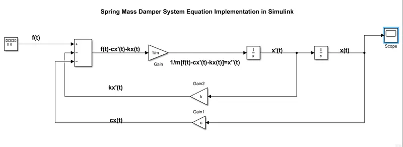
• In the above Model, a Signal Generator has been used to implement the time-dependent External Applied Force on the System. The Waveform selected for the generation of the time-dependent External Applied Force is a Sine Waveform. The Signal emanating from the Signal Generator represents F(t) in the Equation.
• Gain Blocks have been used to represent the Constants k, c and 1/m.
• Integrator blocks have been used to generate x’ and x from x’’.
• Add Block has been used to perform the Add/Subtract Operations as present in the Final Equation.
• The values of the Constants m, c and k have been initialised in the Command Window of the main MATLAB Window. The Simulink Model adheres to the initialisations in the Command Window to initialise the Constants in the Simulink Model.

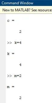
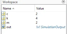
Initializing Constants in the MATLAB Command Window Initialized Constants in the MATLAB Workspace

• The Scope Window has been connected to the signal representing x(Displacement) to get Result of the Model once it has completed Running. The term x(t) also represents the solution of the Basic Spring-Mass-Damper Equation due to Forced Vibrations.

Result:

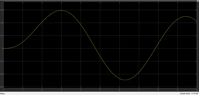
Solution of x(Displacement of mass 'm') w.r.t. Simulation Time

Solution to Objective 3:

For this Objective, a Control Logic has to be implemented in Simulink using Stateflow and the Working of the Logic has to be shown.

The Conditions for the Working of the Traffic Signal as per the Question is as follows:

• RED Light is the default entry state (Entry value at RED state is 1 & Exit Value is 0).
• YELLOW light becomes active after 5 seconds (Entry value at YELLOW state is 1 & Exit Value is 0).
• GREEN Light becomes active after 2 seconds (Entry value at GREEN state is 1 & Exit Value is 0).
• Signal Exits GREEN state to RED state after 5 seconds.

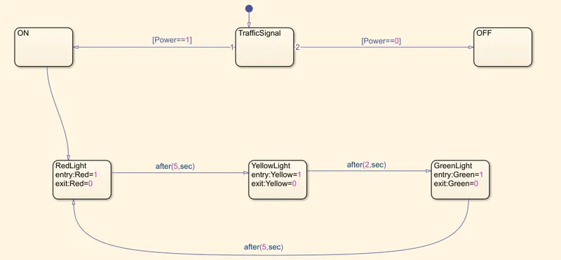
The Control Logic Implemented using Stateflow is as follows:

• In the 1^st State named ‘TrafficSignal’ will first check whether the its succeeding Process will have Power ON or OFF.
• If Boolean Value of Power==0, then the Process ends at OFF State else if the Boolean Value of Power==1, then the Process moves on to the Light Display States (Red, Yellow, Green).
• When the Boolean Value of Power==1, then the process moves on to the RedLight State which according to the Question, has been initialised with Boolean Value of 1 at entry Condition and Boolean Value of 0 at exit condition, i.e. when the Process moves on to the next State, the Boolean Value of the this ‘Redlight’ State becomes 0.
• According to the Question, the Signal becomes Yellow after 5 seconds of Signal being Red. Thus the Process moves on from the ‘RedLight’ State to ‘YellowLight’ State with an exit value of the ‘RedLight’==0. As the ‘YellowLight’ State gets activated after 5 seconds, where according to the Question has been initialised with 1 at entry Condition and Boolean Value of 0 at exit condition, i.e. when the Process moves on to the next State, the Boolean Value of the this ‘YellowLight’ State becomes 0.
• According to the Question, the Signal becomes Green after 2 seconds of Signal being Yellow. Thus the Process moves on from the ‘YellowLight’ State to ‘GreenLight’ State with an exit value of the ‘YellowLight’==0 after 2 seconds. As the ‘GreenLight’ State gets activated after 2 seconds, where according to the Question has been initialised with 1 at entry Condition and Boolean Value of 0 at exit condition, i.e. when the Process moves on to the next State, the Boolean Value of the this ‘GreenLight’ State becomes 0.
• According to the Question, the Signal becomes Red again after 5 seconds of Signal being Green. Thus the Process moves on from the ‘GreenLight’ State to ‘RedLight’ State with an exit value of the ‘GreenLight’==0 after 5 seconds. As the ‘RedLight’ State gets activated after 5 seconds, the Cycle continues as long as the Boolean Value of Power stays 1.
• The Power Variable has been implemented as Input Port to the Stateflow Chart and the ‘RedLight’, ‘GreenLight’ and ‘YellowLight’ State(s) have been implemented as Output Ports from the Stateflow Chart.

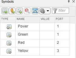
Port Implementation of Stateflow Variables

In the Main Simulink Window, the Input Signal to the Stateflow Chart which represents the ‘Power’ of the Traffic Signal is input using a Constant Block.

The Output Signals from the Stateflow Chart represents the Boolean Value of the Red Light, Yellow Light and the Green Light. The Signals have been connected to their respective Display Blocks which displays the Boolean Values corresponding to the Lights at a given point of time.

These Output Signals are connected to corresponding Lamp Blocks. The Lamp Blocks have been parameterized such that their respective colors gets activated/glows in the Blocks whenever the Boolean Values from these signals returns 1 at a given point of time as per description in the Stateflow Chart.

The Input Signal which represents the Power to the Traffic Signal is controlled by a Toggle Switch Block. Whenever the Toggle Switch is turned OFF, the Boolean Value of the Input Signal becomes 0.

The Simulink Model to implement the Traffic Signal Logic & Function is as follows:

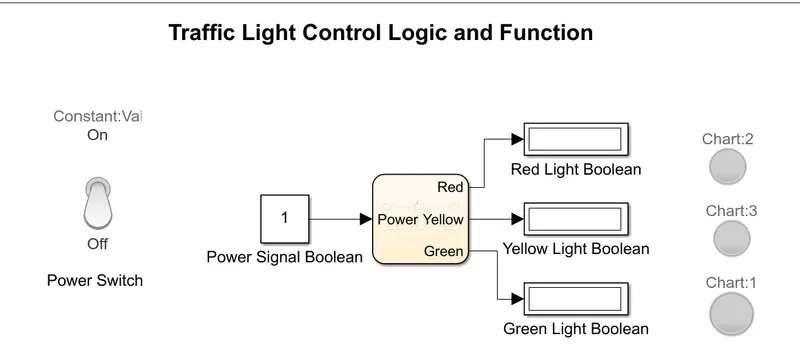
Result: The Simulation Time is set to 20 seconds and the following Observations are made:

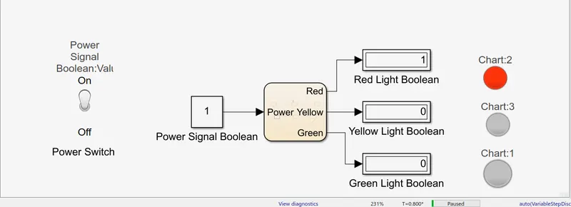
Simulation Result at Simulation Time T=0.800 seconds

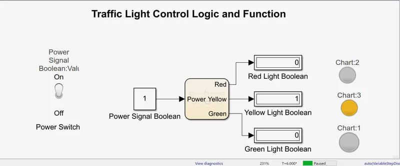
Simulation Result at Simulation Time T=6.000 seconds

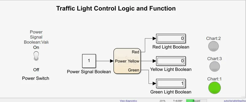
Simulation Result at Simulation Time T=8.000 seconds

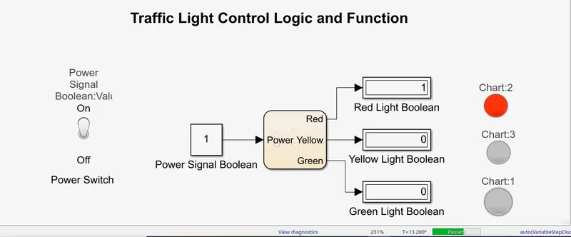
Simulation Result at Simulation Time T=13.200 seconds

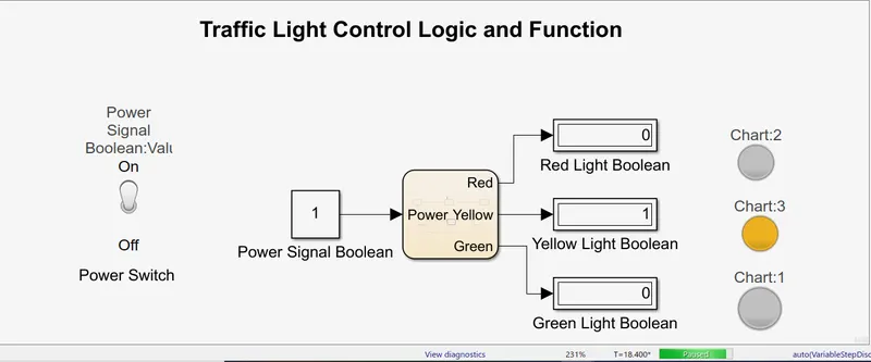
Simulation Result at Simulation Time T=18.400 seconds