Week 8 - Simulating Cyclone separator with Discrete Phase Modelling
Aim: Simulating Cyclone separator with Discrete Phase Modelling
Introduction:
A discrete phase model (DPM) is used when the aim is to investigate the behavior of the particles from a Lagrangian view and a discrete perspective. The fluid phase is treted as continuum by solving Navier-Stokes equation and dispersed or descrete phase is solved by tracking large no of particles, bubbles or droplets through calculated field. At the same time dispersed or descrete phase can exchange mass, momentum and energy with fluid or continuum phase. In the discrete phase model, the assumption is that, discrete phase occupies less volume fraction (less than 10%) compared to fluid phase. The particles trajectories are calculated while calculating fluid flow field. Ansys Fluent predicts the trajectories of discrete phase by integrating force balance on particle.
Following is the calculation procedure followed in the DPM.
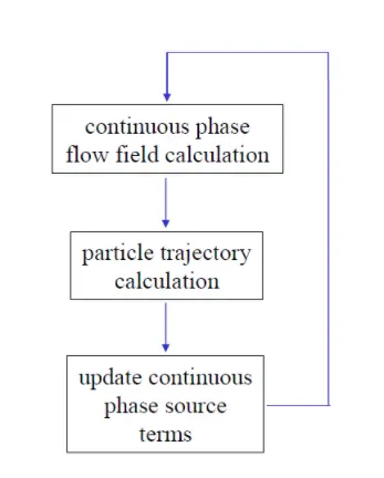
Coupling between continues and discrete phase.
1) One way coupling:
The fluid phase influence the discrete phase via drag and turbulance. On the other hand discrete phase has no influence on fluid phase.
2) Two way coupling:
In this coupling both the phases influence each other. The fluid phase influence the discrete phase via drag and turbulance. And discrete phase influence the fluid phace via sourse terms of mass, momentum and Energy.
Different boundary conditions used in DPM
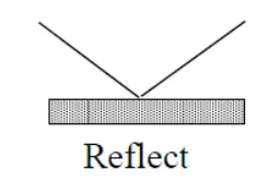
1) Reflect boundary condition
This boundary condition represents that particle rebounds from the boundary, as shown below.
2) Trap boundary condition
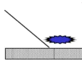
Trap is a type of boundary where trajectory calculations are terminated and particle is considered as trap.
3) Escape boundary condition
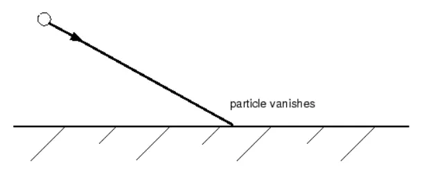
The particle is said to be escaped when it encounters a boundary and trajectory calculations are terminated.
4) Wall film boundary condition
This boundary condition has 4 regimes stick, rebound, spread and splash which are based on impact energy and temperature.
5) Interior boundary condition
This condition means that the particle is passing through internal boundary.
Introduction to cyclonic saperator
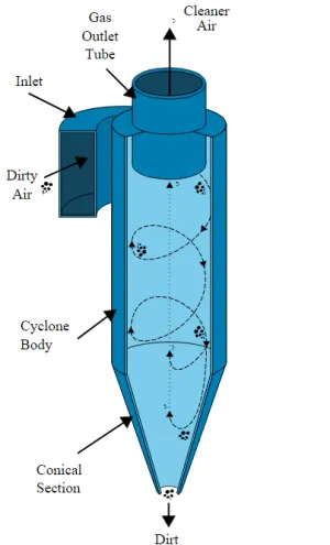
Cyclone separators or simply cyclones are separation devices that use the principle of inertia to remove particulate matter from flue gases. Cyclone separators is one of many air pollution controll devices known as precleaners since they generally remove larger pieces of particulate matter. This prevents finer filtration methods from having to deal with large, more abrasive particles later on. In addition, several cyclone separators can operate in parallel, and this system is known as a multicyclone.
Working principle of cyclonic saperator
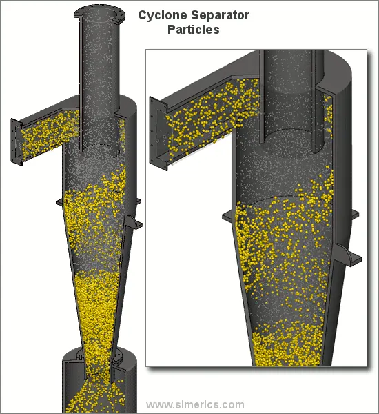
As shown in diagram below, the gas enters the saperator. Gas contains some particles which needs to be saperated out from saperator. As gas enters the saperator, gas is subjected to centrifugal force and vortex like motion is creted as in centrifugal pump. As gas particles are having less inertia, they rises and escape out from top outlet. But the the particles which needs to be saperated (shown in yellow colour) out has more inertia. Due to more inertia, they moves down. In this way saperation occurs in cyclonic saperator.
Four empirical models used to calculate the cyclone separator efficiency
1. Iozia and Leith Model
Iozia and Leith logistic model is a modified version of Barth Model, which is developed based on force balance. The model assumes that a particle carried by the vortex endures the influence of two forces: a centrifugal force, Z and a flow resistance, W. The collection efficiency ηi of particle diameter dpi can be calculated from
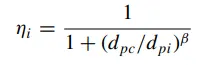
β is an expression for slope parameter derived based on the statistical analysis of experimental data of a cyclone with D = 0.25 m given as

and dpc is the 50% cut size given by Barth.
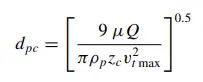
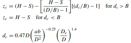
where core length, zc, and core diameter, dc, are given as
2. Li and Wang Model
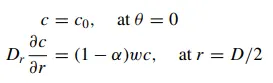
The Li and Wang model includes particle bounce or reentrainment and turbulent diffusion at the cyclone wall. A twodimensional analytical expression of particle distribution in the cyclone is obtained. Li and Wang model was developed based on the following assumptions:
• The radial particle velocity and the radial concentration profile are not constant for uncollected particles within the cyclone.
• Boundary conditions with the consideration of turbulent diffusion coefficient and particle bounce reentrainment on the cyclone wall are:
The tangential velocity is related to the radius of cyclone by

The concentration distribution in a cyclone is given as
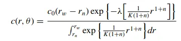
where
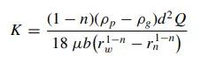
and
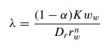
The resultant expression of the collection efficiency for particle of any size is given as
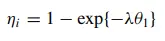
Where
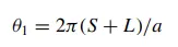
3. Koch and Licht Model
Koch and Licht collection theory recognized the inherently turbulent nature of cyclones and the distribution of gas residence times within the cyclone. Koch and Licht described particle motion in the entry and collection regions with the additional following assumptions:
• The tangential velocity of a particle is equal to the tangential velocity of the gas flow, i.e. there is no slip in the tangential direction between the particle and the gas.
• The tangential velocity is related to the radius of cyclone by:

A force balance and an equation on the particles collection yields the grade efficiency ηi

Where,
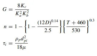
G is a factor related to the configuration of the cyclone, n is related to the vortex and τ is the relaxation term.
4. Lapple Model
Lapple model was developed based on force balance without considering the flow resistance. Lapple assumed that a particle entering the cyclone is evenly distributed across the inlet opening. The particle that travels from inlet half width to the wall in the cyclone is collected with 50% efficiency. The semi empirical relationship developed by Lapple to calculate a 50% cut diameter, dpc, is
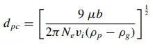
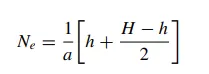
where Ne is the number of revolutions
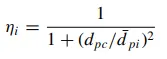
The efficiency of collection of any size of particle is given by
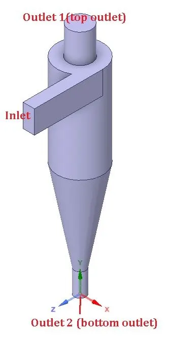
Model of cyclonic saperator used in CFD analysis
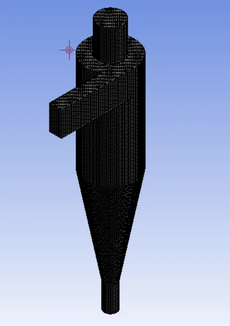
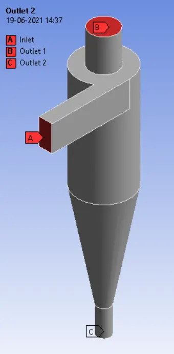
Model has inlet and 2 outlets, one is at top and another is at bottom.
Meshing of a model
Type of Mesh: Body fitted cartesian mesh
Element size: 5 mm
No. of nodes: 456576
No. of elements: 427841
Named selections
Simulation is performed for following 2 cases
1) Variable particle diameter (1 µm, 2µm, 3µm, 4µm and 5µm) and constant velocity of 3 m/sec
2) variable particle velocity (1 m/sec, 2m/sec, 3m/sec, 4m/sec, and 5m/sec) and constant particle diameter of 5 µm
Simulation settings
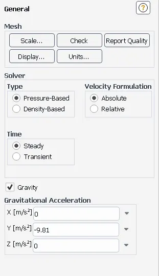
A) General settings
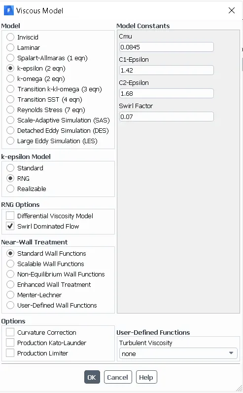
B) Viscous models
C) Descrete phase modelling
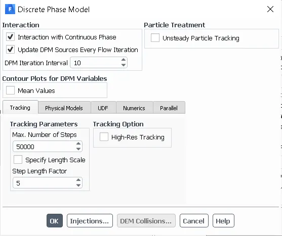
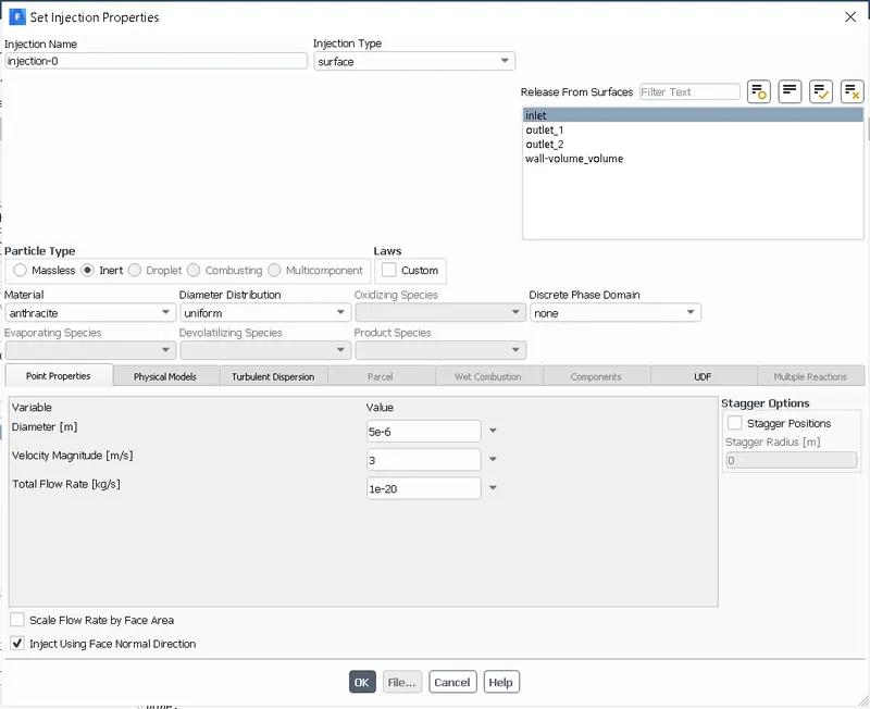
D) Boundary conditions
a) Inlet: Velocity inlet and reflect decrete phase boundary type
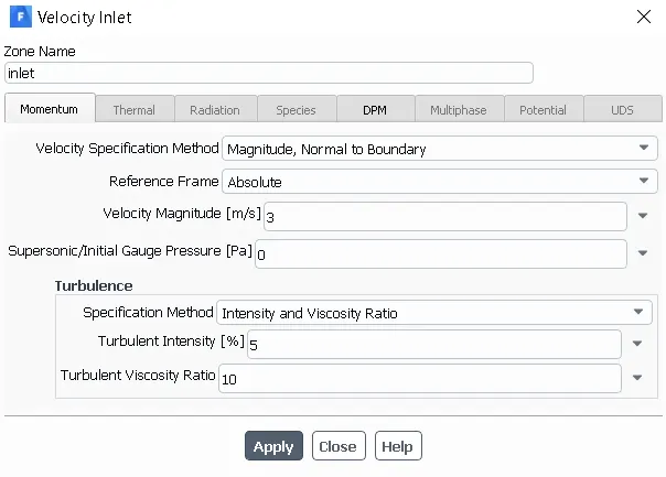
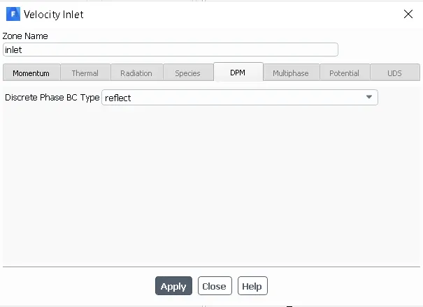
b) Top outlet: Pressure outlet and escape descrete phase boundary type
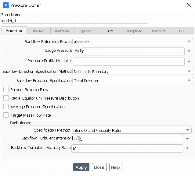
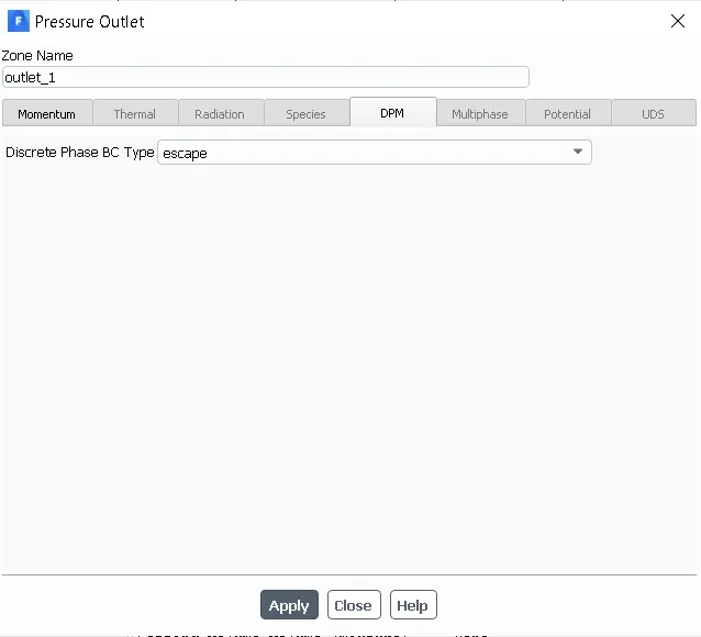
c) Bottom outlet: Pressure outlet and trap descrete phase boundary type
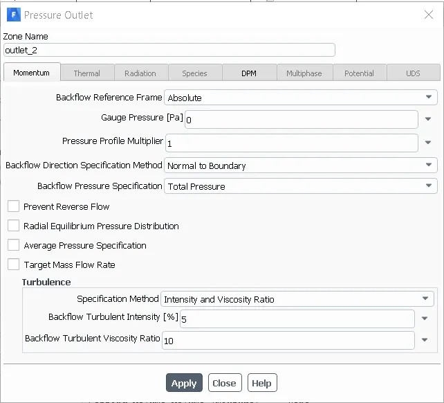
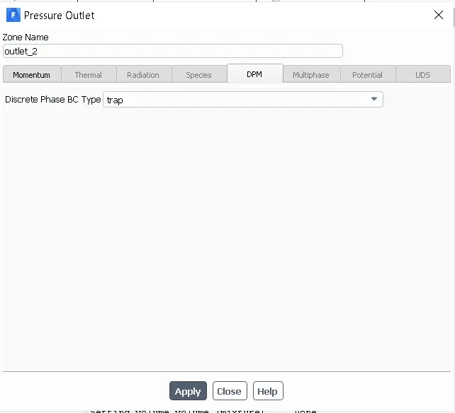
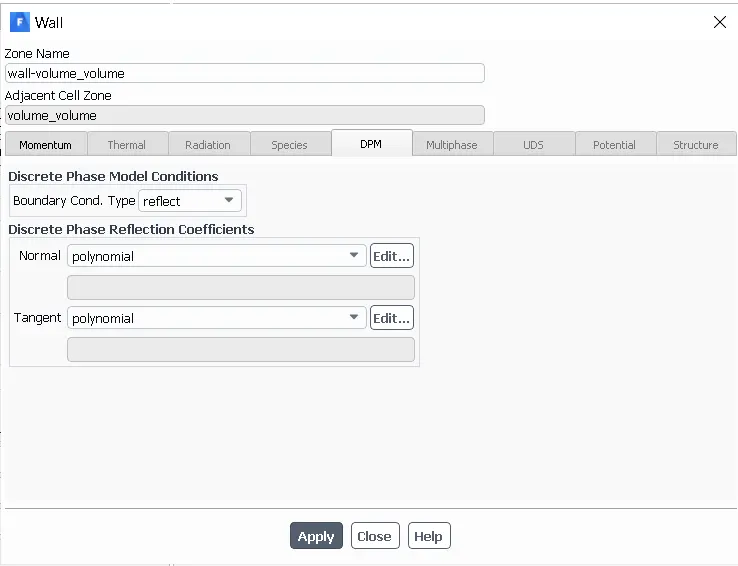
d) Wall: Wall and reflect decrete type boundary
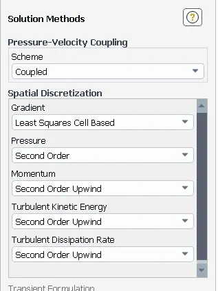
E) Solution methods
A) Results for variable particle diameter and constant velocity of 3 m/sec
1) Partcle diamter 1 µm
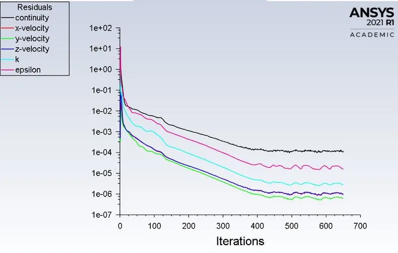
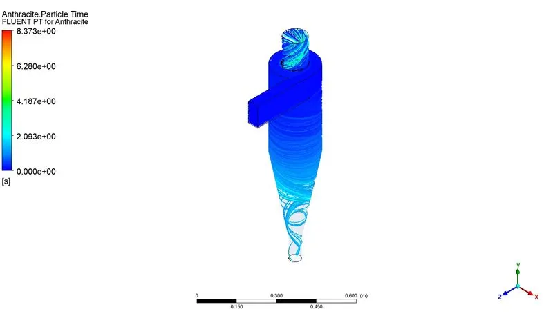
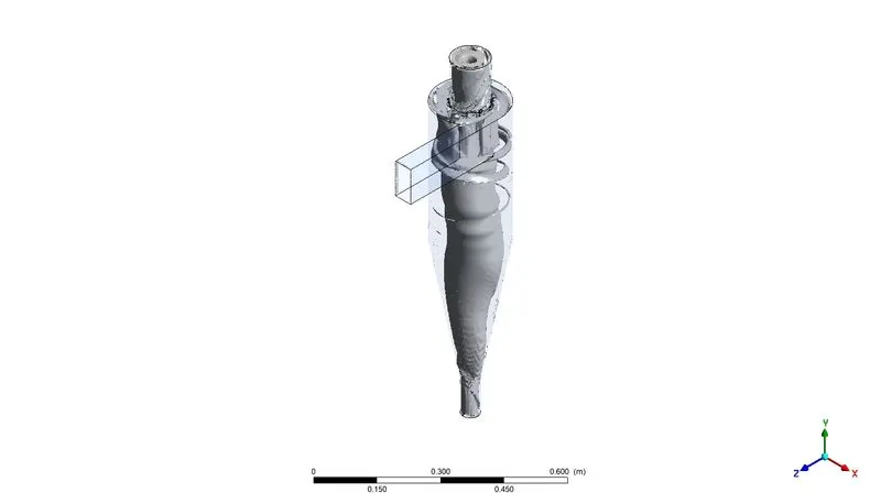

Saperator Efficiency = No of partcles trapped/No of partcles tracked = 126/378 = 33.33%
Animation: https://drive.google.com/file/d/1gG_rUGaGso0hNG6vWU821hMKVOQ7rNug/view?usp=sharing
2) Partcle diamter 2 µm
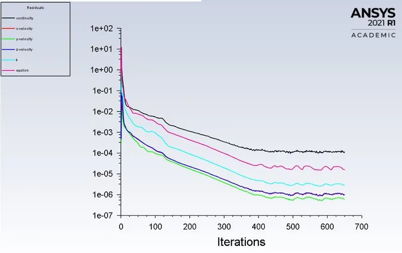
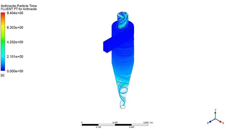

Saperator Efficiency = No of partcles trapped/No of partcles tracked = 131/378 = 34.65%
Animation: https://drive.google.com/file/d/1wxTdT1dl1d6DAWsY9QlHFuaRN4SzxqX-/view?usp=sharing
3) Partcle diamter 3 µm
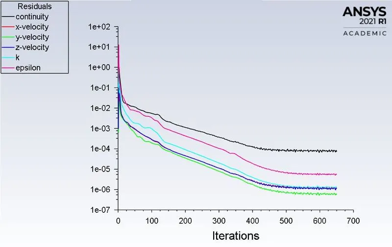
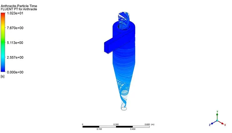
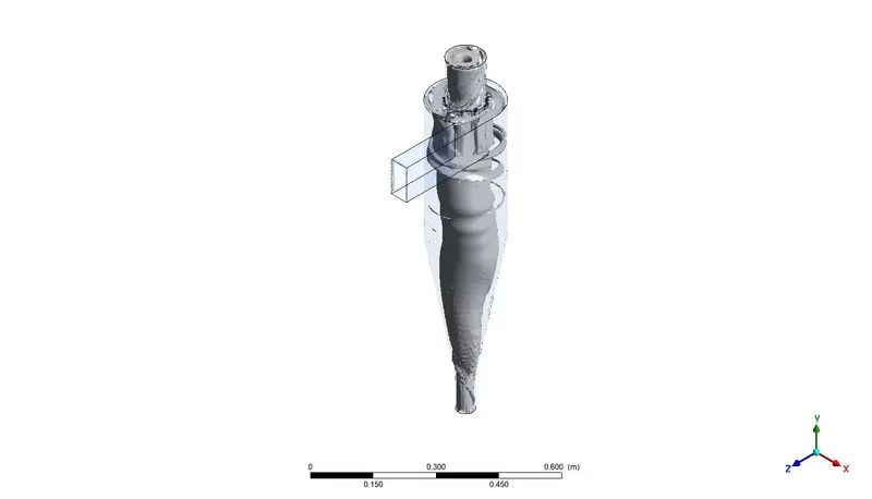

Saperator Efficiency = No of partcles trapped/No of partcles tracked = 152/378 = 40.21%
Animation: https://drive.google.com/file/d/1AzzlvgiPykuVcRPgSYJOGJ02QDhw6t3K/view?usp=sharing
4) Partcle diamter 4 µm
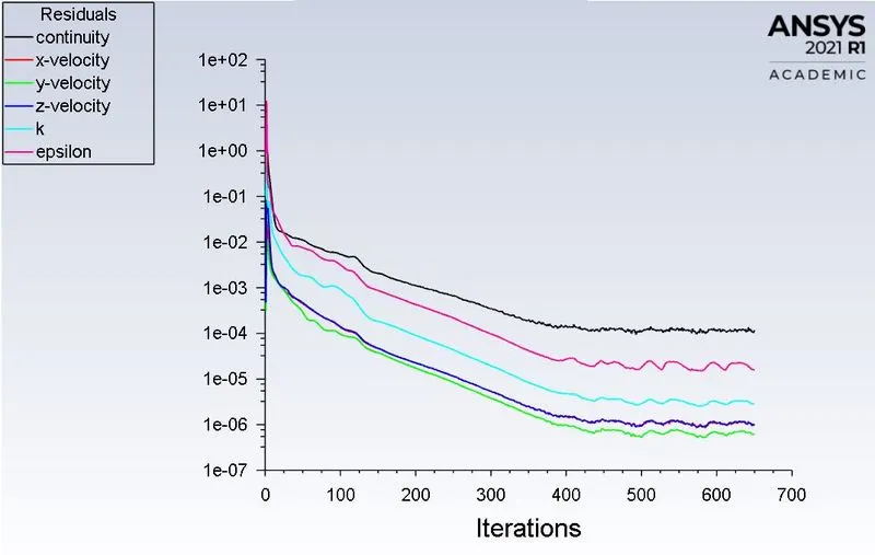
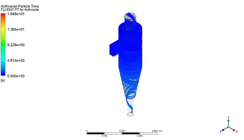

Saperator Efficiency = No of partcles trapped/No of partcles tracked = 190/378 = 50.26%
Animation: https://drive.google.com/file/d/1PBAPleAMAKrQcPmBHcjViSv_5e8dQ3pj/view?usp=sharing
5) Partcle diamter 5 µm
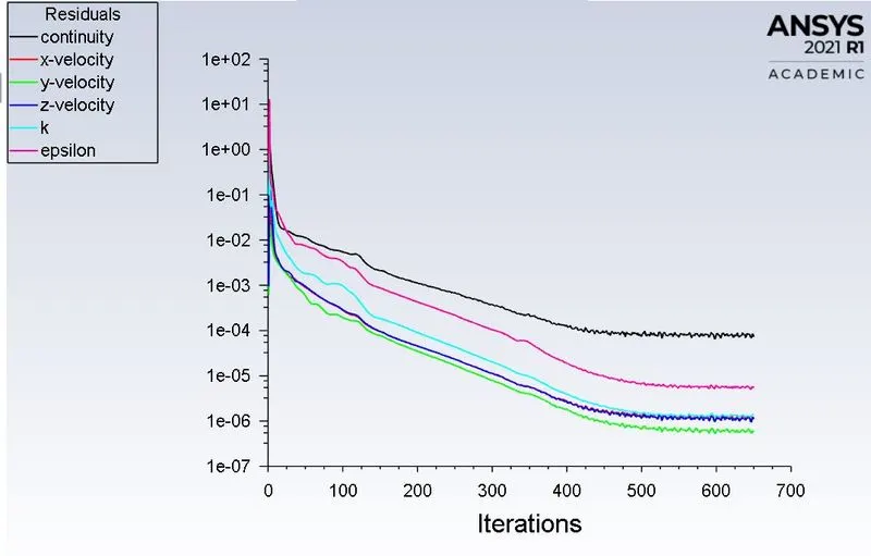
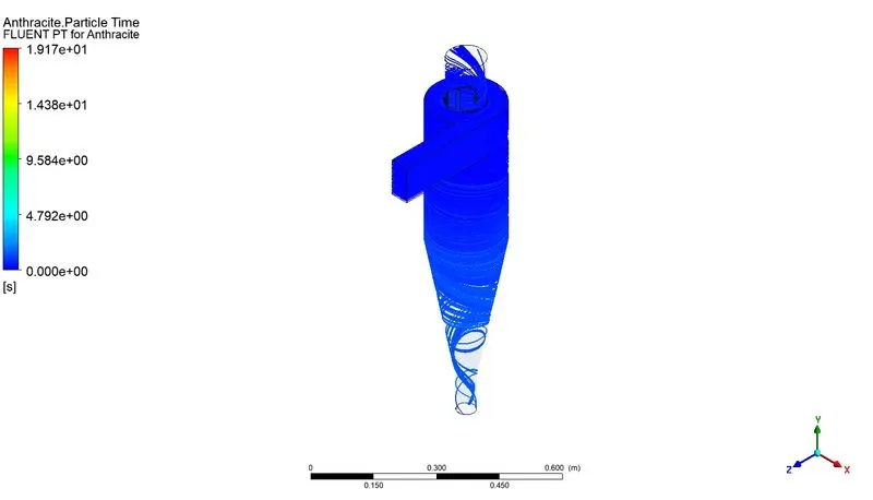

Saperator Efficiency = No of partcles trapped/No of partcles tracked = 180/378 = 47.61%
Animation: https://drive.google.com/file/d/1EnnORrxzdedkvVksdjoE-shEys7yTrex/view?usp=sharing
B) Results for variable particle velocity and constant particle diameter of 5 µm
1) Particle velocity 1 m/sec
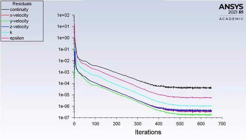
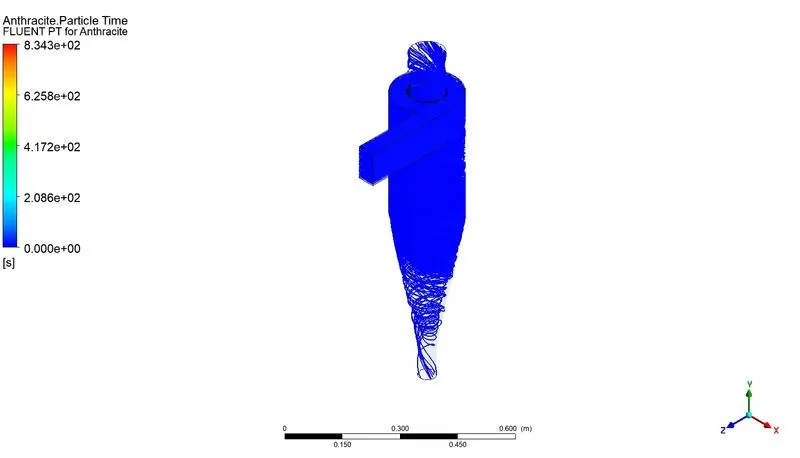
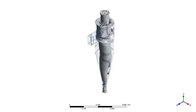

Saperator Efficiency = No of partcles trapped/No of partcles tracked = 8/378 =2.11%
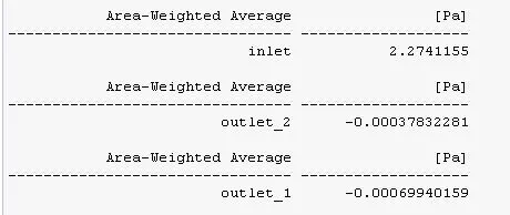
Static pressure drop from inlet to top outlet (outlet 1) = 2.2748 Pa
Static pressure drop from inlet to bottom outlet (outlet 2) = 2.2744 Pa
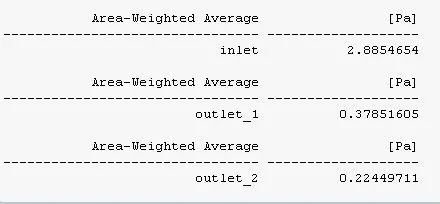
Total pressure drop from inlet to top outlet (outlet 1) =2.5069 Pa
Total pressure drop from inlet to bottom outlet (outlet 2) = 2.6609 Pa
Animation: https://drive.google.com/file/d/1ChdzZwl7fjSnOGepJ2pnxcP2cm7Na1Ed/view?usp=sharing
2) Particle velocity 2 m/sec
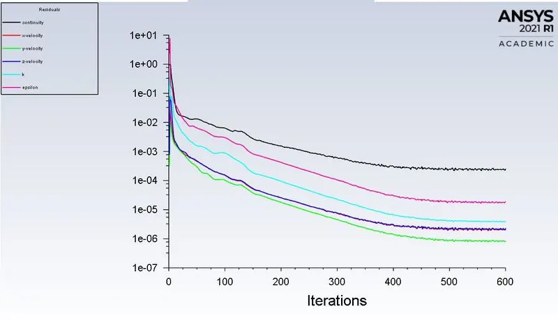
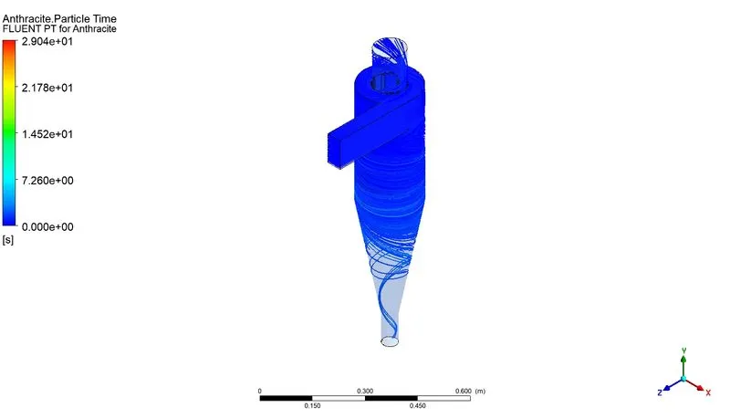
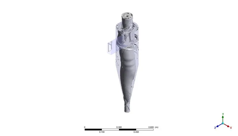

Saperator Efficiency = No of partcles trapped/No of partcles tracked = 18/378 =4.76%
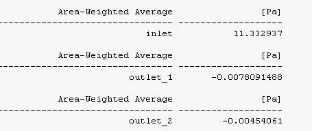
Static pressure drop from inlet to top outlet (outlet 1) = 11.3707 Pa
Static pressure drop from inlet to bottom outlet (outlet 2) = 11.3374 Pa
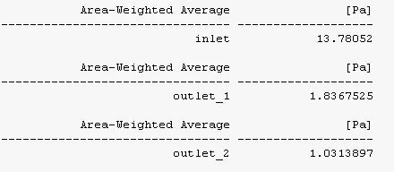
Total pressure drop from inlet to top outlet (outlet 1) =11.9437 Pa
Total pressure drop from inlet to bottom outlet (outlet 2) = 12.7491 Pa
Animation: https://drive.google.com/file/d/1vByDYoTRzPx6pxWEBp7ptDjQTh5LokCf/view?usp=sharing
3) Particle velocity 3 m/sec
Saperator Efficiency = No of partcles trapped/No of partcles tracked = 180/378 =47.61%
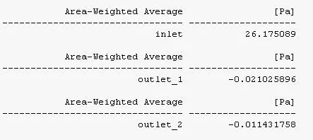
Static pressure drop from inlet to top outlet (outlet 1) = 26.1961 Pa
Static pressure drop from inlet to bottom outlet (outlet 2) = 26.1865 Pa
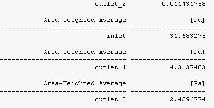
Total pressure drop from inlet to top outlet (outlet 1) =27.3695 Pa
Total pressure drop from inlet to bottom outlet (outlet 2) = 29.22 Pa
Animation: https://drive.google.com/file/d/10qGGdESI7litTNBffCodhfFfk0ecr0_3/view?usp=sharing
4) Particle velocity 4 m/sec
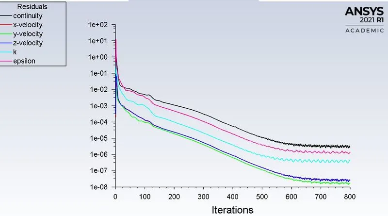
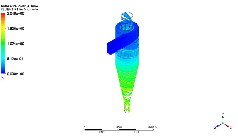
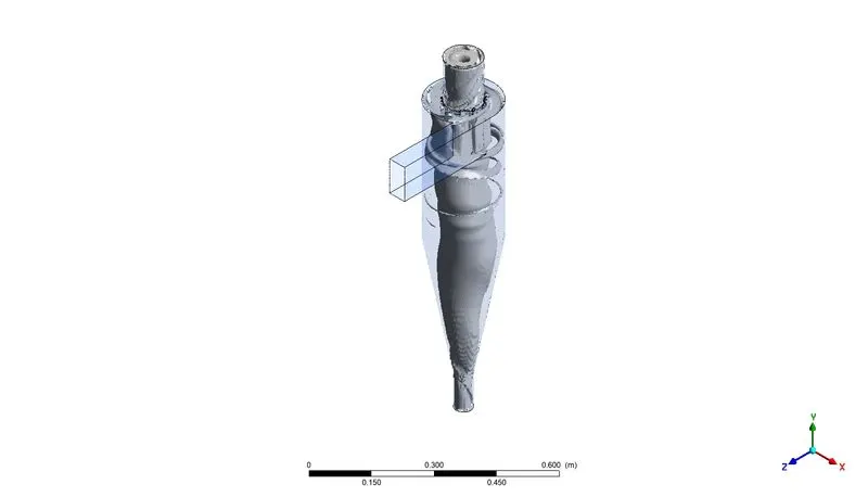

Saperator Efficiency = No of partcles trapped/No of partcles tracked = 313/378 =82.8%
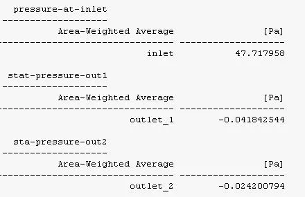
Static pressure drop from inlet to top outlet (outlet 1) = 47.7559 Pa
Static pressure drop from inlet to bottom outlet (outlet 2) = 47.7421 Pa
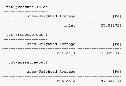
Total pressure drop from inlet to top outlet (outlet 1) = 49.6093 Pa
Total pressure drop from inlet to bottom outlet (outlet 2) = 53.0196049 Pa
Animation: https://drive.google.com/file/d/1PAC-R-Wo0vaUIYCdGPel-5tgBIq2DxjG/view?usp=sharing
5) Particle velocity 5 m/sec
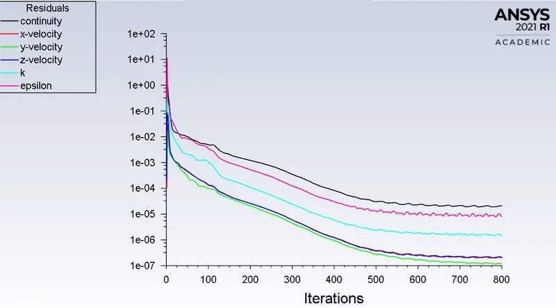
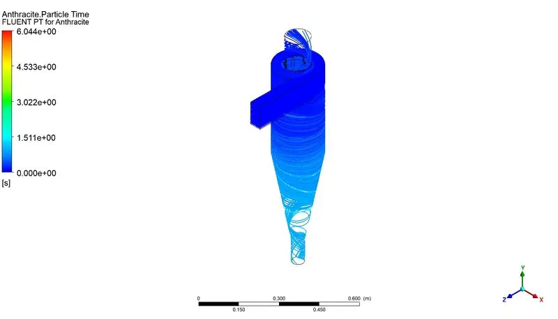
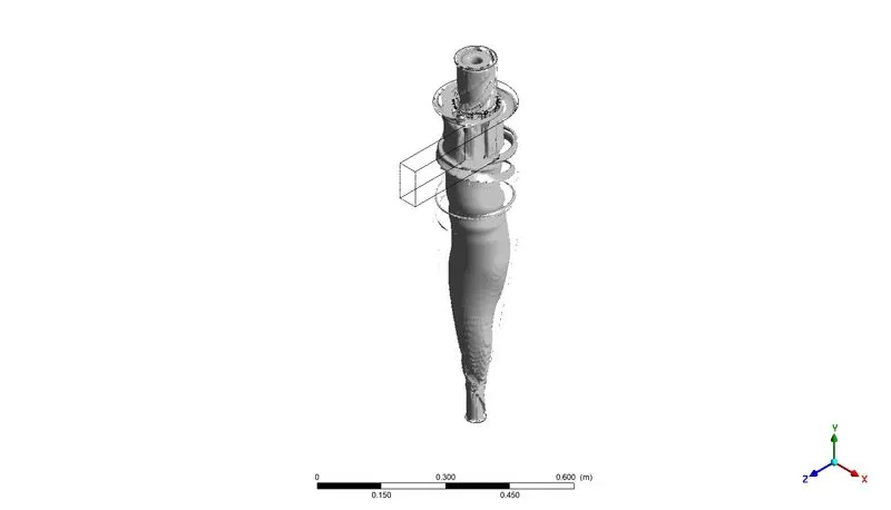

Saperator Efficiency = No of partcles trapped/No of partcles tracked = 283/378 =74.86%
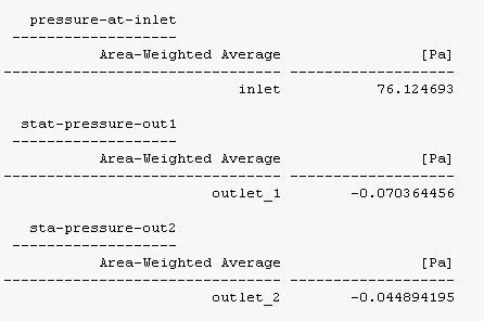
Static pressure drop from inlet to top outlet (outlet 1) = 76.19505 Pa
Static pressure drop from inlet to bottom outlet (outlet 2) = 76.1695 Pa
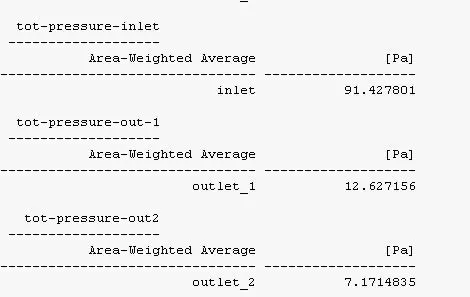
Total pressure drop from inlet to top outlet (outlet 1) = 78.8 Pa
Total pressure drop from inlet to bottom outlet (outlet 2) = 84.2563 Pa
Animation: https://drive.google.com/file/d/1YEsy_o3A2sglOu_XuU3lPdHL9-zW_IZt/view?usp=sharing
Discussion:
1)Variable particle diameter and constant velocity (3 m/sec)
| Sr. No | Particle diameter (µm) |
Saperation efficiency of cyclonic saperator (%) |
| 1 | 1 | 33.33 |
| 2 | 2 | 34.65 |
| 3 | 3 | 40.21 |
| 4 | 4 | 50.26 |
| 5 | 5 | 47.61 |
From above table it is found that, as particle diamter increases, cyclonic saperator efficiency increses.
2) Variable velocity and constant particle diameter (5 µm)
| Sr. No | Particle velocity (m/sec) |
Saperation efficiency of cyclonic saperator (%) |
Static pressure drop from inlet to outlet 1 (Top outlet) (Pa) |
Total pressure drop from inlet to outlet 1 (Top outlet) (Pa) |
| 1 | 1 | 2.11 | 2.27 | 2.50 |
| 2 | 2 | 4.76 | 11.37 | 11.94 |
| 3 | 3 | 47.61 | 26.19 | 27.36 |
| 4 | 4 | 82.8 | 47.75 | 49.60 |
| 5 | 5 | 74.86 | 76.16 | 78.8 |
From above table it is found that,
- As particle velocity increses, separation efficiency also increses except in case of 5 m/sec velocity
- As particle velocity increses, both static and total pressure drop increases.