Week 5 - Rayleigh Taylor Instability
Aim: Simulation of Rayleigh Taylor (RT) instability phenomenon
Theory: RT instability phenomena occurs at the interface of two fluids of different densities, when lighter fluids pushing the heavier fluid. It is a dynamic process whereby the two fluids seek to reduce their combined potential energy.This phenomena occurs when heavy fluid is placed over lighter fluid. For example dense water over oil (liquid–liquid), or water over air(gas–liquid).
Following are some practical CFD models that have been based on the mathematical analysis of Rayleigh Taylor waves.
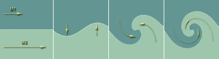
1) Kelvin–Helmholtz instability:
The Kelvin–Helmholtz instability typically occurs when there is velocity shear in a single continues fluid, or additionally where there is a velocity difference across the interface between two fluids. For example when wind blows across a water surface.
2) Richtmyer–Meshkov instability:
The Richtmyer–Meshkov instability (RMI) occurs when two fluids of different density are impulsively accelerated.
3) Plateau–Rayleigh instability:
The Plateau–Rayleigh instability, explains why and how a falling stream of fluid breaks up into smaller packets with the same volume but less surface area.
Simulation of Rayleigh Taylor Instability
Simulation is carried out for baseline mesh where element size is 0.5 mm. Then simulation is carried out with refined mesh and effect of mesh size is studied on results are studied. After this simulation is carried out with refine mesh for water and user difned fluid.
Geometry/Model used in the simulation
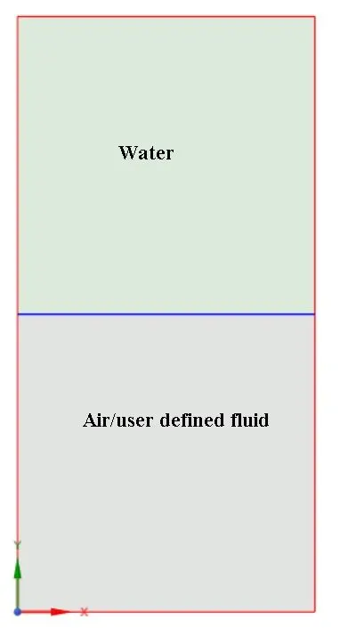
The model consist of two squares of 20 mm x 20 mm dimentions with interface between them. Upper square containes water and lower square containes air or user defined material.
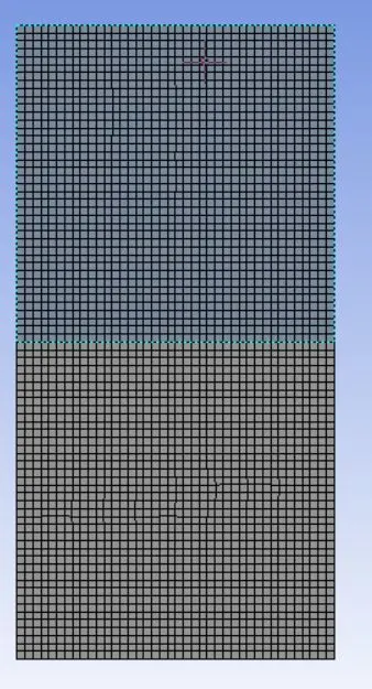
1) Simulation with baseline mesh (Element size = 0.5 mm)
No of elements = 3200
Simulation Results:
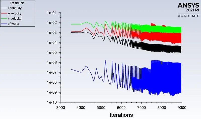
Animation of volume fraction of water:
https://drive.google.com/file/d/1SOAfq2nEeEphcaLupTDRC-Ea0xcZ2Rr8/view?usp=sharing
2) Simulation with elememt size = 0.3 mm
No of elements = 8978
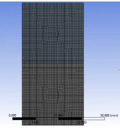
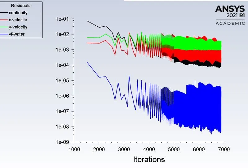
Animation of volume fraction of water:
https://drive.google.com/file/d/1UYDwH_lt6b_FGsUT29QOnHOjQZLyeeC6/view?usp=sharing
3) Simulation with elememt size = 0.2 mm
No of elements =20000
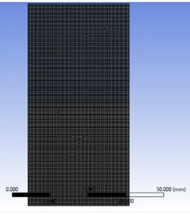
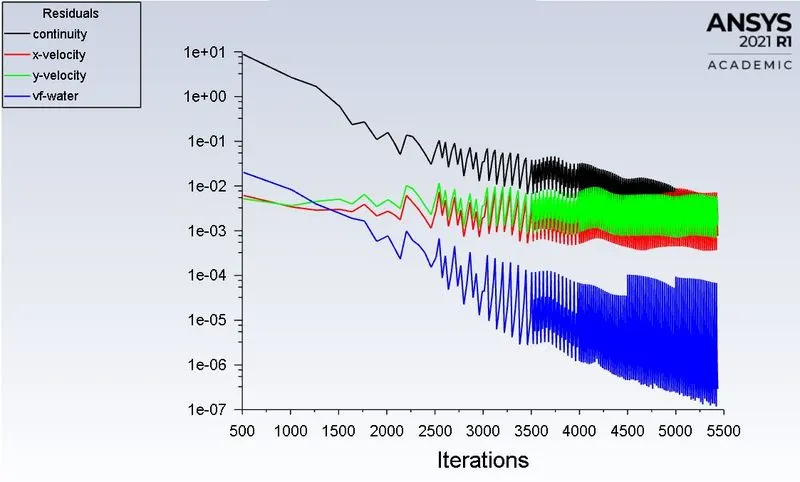
Animation of volume fraction of water:
https://drive.google.com/file/d/1-WY1v4HIsb6Ag9xS0kvNpdmQDrO1veaP/view?usp=sharing
4) Simulation with user defined fluid
Mesh with element size 0.2 mm is used for this simulation
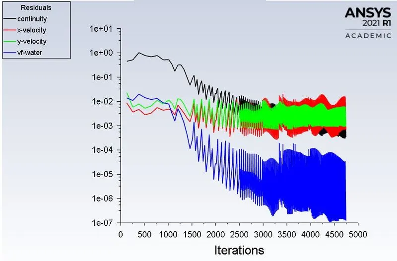
Animation of volume fraction of water:
https://drive.google.com/file/d/1_R_KnGjzQfidfq4WN-tG_tW1dc66o9zL/view?usp=sharing
Atwood No:
Atwood number (A) is dimentionless number in study of hydrodynamic instabilities in density stritified flows.
It is defined as,
`A = (rho1 -rho2)/(rho1+rho2)`
Where `rho1 and rho2` are the densities of heavier and lighter fluids
In case of water and air,
`A = (998.2-1.225)/(998.2+1.225)=0.9975`
In case of water and user defined fluid
`A = (998.2-400)/(998.2+400)=0.4278`
Magnitude of atwood number affects the bahaviour of fluids when they interact with each other. As can be seen from animations.
Effects of mesh refinement on simulation
As mesh is refined the results are much smoother as can be seen from results with mesh size of 0.5 mm, 0.3 mm and 0.2 mm. With reduction in mesh size the instability contours are much smoother and formation of bubbles and its motion is much clearly visible.
In this simulation steady state approach is not possible because, with steady state final results we can see. But in this case, we need to observe how instability phenomena works and how the fluid behaviour changes with time. This is possible only with unsteady simulation, as with unsteady simulation, we can see the variations with repect to time rather than just end results.