Week 7 - Simulation of a 1D Super-sonic nozzle flow simulation using Macormack Method
Aim: Simulation of quasi 1 dimentionbal noozle flow using Macormack method.
Objectives:
1. Steady-state distribution of primitive variables inside the nozzle
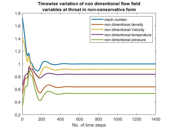
2. Time-wise variation of the primitive variables
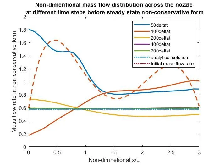
3. Variation of Mass flow rate distribution inside the nozzle at different time steps during the time-marching process
4. Comparison of Normalized mass flow rate distributions of both forms
Introduction to problem/Physical aspects of problem
1D, steady, isentropic flow is considered through Convegent-divergent nozzle. It is assumed that nozzle is connected to a very large reservior whose area is infinite. Hence velocity at inlet to nozzle is zero or neglisible. Pressure and temperature at inlet to nozzle is `p_0`and `T_0`.
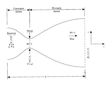
Figure: Nozzle scematic
It is assumed that flow properties are varying along x-diretion only and at section flow properties are constant along y-direction (though it is true in reality).
Analytical solution of problem
Problem is chosen whose analytical solution is known.
Governing equations are
Continuity equation `ρ_1 V_1 A_1= ρ_2 V_2 A_2`
Momentum Equation `ρ_1 V_1+ρ_1 V_1^2 A_1+∫_(A_1)^(A_2)p d A=p_2 A_2+ρ_2 V_2^2 A_2`
Energy Equation `h_1+(V_1^2)/2=h_2+(V_2^2)/2`
Solving above equtions analytically following results are obatained.
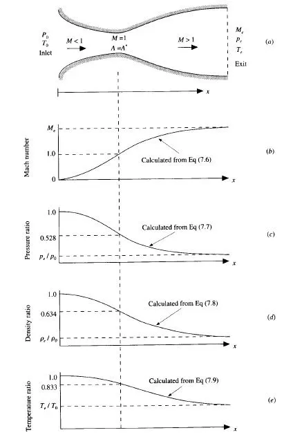
Figure: Analytical results
Solution by using CFD technique
Solution is obtained using both conservation and non-conservation form governing equations
a) Solution using non-conservation form governing equations
Following are the governing equations in non-conservation form
Continuity equation`(∂(ρA))/(∂t)+(∂(ρAV))/(∂x)=0`
Momentum Equation`ρ (∂V)/(∂t)+ρV (∂V)/(∂x)=-(∂p)/(∂x)`
Energy Equation`ρc_v (∂T)/(∂t)+ρVc_v (∂T)/(∂x)=-p (∂V)/(∂x)-pV (∂(ln A))/(∂x)`
Above equations are in dimentional form. In non dimentional form above equtions can be written as,
Continuity equation `(∂ρ^')/(∂t^') =-ρ^' (∂v^')/(∂x^') -ρ^' V^' (∂(ln A^' ))/(∂x^') -V^' (∂ρ^')/(∂x^')`
Momentum Equation`(∂V^')/(∂t^') =-V^' (∂v^')/(∂x^') -1/γ ((∂T^')/(∂x^') +T^'/ρ^' (∂ρ^')/(∂x^' ))`
Energy Equation `(∂T^')/(∂t^') =-V^' (∂T^')/(∂x^') -(γ-1)T^' ((∂V^')/(∂x^') +V^' (∂(lnA^' ))/(∂x^' ))`
Where,
`T^'=T/T_0`, `ρ^'=ρ/ρ_0`, `x^'=x/L` `V^'=V/a_0``t^'=t/((L⁄a_0 ) )``A^'=A/(A*)``p^'=p/p_0`
Please note that all prime quantities are non-domentional in nature.
A* is a throat area and `a_0`is speed of sound in reservior`
Now, to solve above equations by Macormack method ( Predictor step and Corrector step).
a) Predictor step
- Descritisation and solution of governing equations by first order forward difference (to find `((∂ρ)/(∂t))_p, ((∂V)/(∂t))_p ((∂T)/(∂t))_p`)
- To obtaine Predicted values of temperature, density and velocity.`ρ_i^(t+∆t)=ρ_i^t+((∂ρ)/(∂t))_i^t ∆t``V_i^(t+∆t)=V_i^t+((∂V)/(∂t))_i^t ∆t``T_i^(t+∆t)=T_i^t+((∂T)/(∂t))_i^t ∆t`
b) Corrector step
- Descritisation and solution of governing equations by first order forward difference (`((∂ρ)/(∂t))_c, ((∂V)/(∂t))_c ((∂T)/(∂t))_c`).
- To compute average time derivative of temperature, density and velocity. `((∂ρ)/(∂t))_(ave)=0.5[((∂ρ)/(∂t))_p+((∂ρ)/(∂t))_c ]``((∂V)/(∂t))_(ave)=0.5[((∂V)/(∂t))_p+((∂V)/(∂t))_c ]`
`((∂T)/(∂t))_(ave)=0.5[((∂T)/(∂t))_p+((∂T)/(∂t))_c ]`
- To obtain corrected values of temperature, density and velocity.`ρ_i^(t+∆t)=ρ_i^t+((∂ρ)/(∂t))_((avg)) ∆t``V_i^(t+∆t)=V_i^t+((∂V)/(∂t))_((avg)) ∆t``T_i^(t+∆t)=T_i^t+((∂T)/(∂t))_((avg)) ∆t`
Calculation of time step
Time step is clculated for all time step using following expression
`∆t=C ((∆x)/(V+√T))`
Where C = CFL number = 0.5
Time step is clculated for all nodes and minimum of it is taken as time step for further calculations.
Nozzle shape
Nozzle shape is varying parabolically w.r.t. x as `A=1+2.2(x-1.5)^2 for 0≤x≤3`
Initial conditions
Initial condition for density, velocity and temperature are calculated from following expressions
`ρ=1-0.3146 x,T=1-0.146 x and V= (0.1+1.09 x)T^(1/2)`
Boundary conditions
a) Subsonic inflow boundary condition (First node)
`V_1=2V_2-V_3`
b) Supersonic outflow boudary conditions (Last node)
`V_N=2V_(N-1)-V_(N-2)
`ρ_N=2ρ_(N-1)-ρ_(N-2)`
`T_N=2T_(N-1)-T_(N-2)`
b) Solution using non-conservation form governing equations
Continuity equation (Dimentional form)
`(∂(ρA))/(∂t)+(∂(ρAV))/(∂x)=0`
Continuity equation (Non-dimentional form)
`(∂(ρ^' A^'))/(∂t^') +(∂(ρ^' A^' V^'))/(∂x^') =0`
Momentum equation (Dimentional form)
`(∂(ρAV))/(∂t)+(∂(ρAV^2))/(∂x)=-A (∂p)/(∂x)`
Momentum equation (Non-dimentional form)
`(∂(ρ^' A^' V^'))/(∂t^,)+∂/(∂x^') (ρ^' A^' V'^2+1/γ p^' A^' ) =1/γ p^' (∂A^')/(∂x^')`
Energy equation (Dimentional form)
`∂([ρ(e+V^2/2)A])/(∂t)+∂([ρ(e+V^2/2)AV])/(∂x)=-(∂(pAV))/(∂x)`
Energy equation (Non-dimentional form)
`∂([ρ^' (e^'/(γ-1)+γ/2 V^'2 ) A^,])/(∂t^' )+∂[ρ^' (e^'/(γ-1)+γ/2 V^'2 ) V^' A^'+ρ^' A^' V^' ]/(∂x^') =0`
Now Let us define elements of solution vector U, the solution vector F and the source term J as follows
`U_1=ρ^' A^'`
`U_2=ρ^' A^' V^'`
`U_3=ρ^' (e^'/(γ-1)+γ/2 V'^2 ) A^'`
`F_1=ρ^' A^' V^'`
`F_2=ρ^' A^' V'^2+1/γ p^' A^'`
`F_3=ρ^' (e^'/(γ-1)+γ/2 V'^2 ) V^' A^'+p^' A^' V^'`
`J_2=1/γ p^' ((∂A^')/(∂x^') )`
Substituting above equations in governing differential equation we get
`(∂U_1)/(∂t^') = -(∂F_1)/(∂x^')`
`(∂U_2)/(∂t^') = -(∂F_2)/(∂x^,)+J_2`
`(∂U_3)/(∂t^') = -(∂F_3)/(∂x^,)`
Above equations are governing differential equations for quasi one dimentional flow in conservation form.
Now, from definations U1, U2 and U3
`ρ^'=U_1/A^'`
`V^'=U_2/U_1`
`T^'=e^'=(γ-1)(U_3/U_1 -γ/2 V'^2 )`
`p^'=ρ^' T^'`
Now,
`F_1=U_2`
`F_2=(U_2^2)/U_1 +(γ-1)/γ (U_3-γ/2 (U_2^2)/U_1 )`
`F_3=γ (U_2 U_3)/U_1 -γ(γ-1)/2 (U_2^3)/(U_1^2 )`
`J_2=(γ-1)/γ (U_3-γ/2 (U_2^2)/U_1 ) ∂((ln A^') )/(∂x^')`
Initial conditions
For `0≤x^'≤0.5 ,ρ^'=1,T^'=1`
For `0.5≤x^'≤1.5 ,ρ^'=1-0.366(x^'-0.5),T^'=1-0.167(x^'-0.5)`
For `1.5≤x^'≤3.5 ,ρ^'=0.634-0.3879(x^'-1.5), T^'=0.833-0.3507(x^'-1.5)`
Nozzle shape
`A=1+2.2(x-1.5)^2 for 0≤x≤3`
`U_1=ρ^' A^'`
`U_2=ρ^' A^' V^,`
`U_3=ρ^' (e^'/(γ-1)+γ/2 V'^2 ) A^'`
`V^'=U_2/(ρ^' A^' )`
Boundary conditions
a) Subsonic inflow boundary condition (First node)
`(U_1 )_(i=1)=(ρ^' A^' )_(i=1)=A_(i=1)^'`=Fixed value
`(U_2 )_(i=1)=2(U_2 )_(i=2)-(U_2 )_(i=3)`
`U_3=U_1 (T^'/(γ-1)+γ/2 V'^2 )`
b) Supersonic outflow boudary conditions (Last node)
`(U_1 )_N=2(U_1 )_(N-1)-(U_1 )_(N-2)`
`(U_2 )_N=2(U_2 )_(N-1)-(U_2 )_(N-2)`
`(U_3 )_N=2(U_3 )_(N-1)-(U_3 )_(N-2)`
Main code
clear all
close all
clc

% Inputs
n=31;
L=3;
x= linspace(0,L,n);
dx=x(2)-x(1);
gamma = 1.4;
c=0.5;
nt=1400;
m_analytical = 0.579*ones(n);

    tic
%  Solving the governing equations in non-conservative form
     [x,dt,rho,v,t,p,M,flow_rate_n,nt_grid,nn_iter] = non_conservative_part(L,n,c,dx,nt);
     time_nc=toc;

    tic
  % Solving the governing equations in conservative form
    [dt, rho,t,p,M,v,flow_rate,m_analytical,cn_iter,tolerance] = conservative_part(L,n,c,dx,gamma,nt);
    time_c=toc;

% To compare mass flow rates
 figure(7)
 plot(x,flow_rate_n,'Linewidth',2)
 hold on
 plot(x,flow_rate,'Linewidth',2)
 hold on
 plot(x, m_analytical, 'linewidth',2)
 legend('Non-conservative form','Conservative form','Analytical solution')
 xlabel('Non-demention length (x/L)')
 ylabel('Mass flow rate')
 title({'Comparison of mass flow rate'})

  % To compare convergance rate in Conservative and Non-conservative form
 figure(8)
 time = [time_nc time_c];
 x = [1 2];
 bar(x, time)
 xlabel('1. Non-conservative approach 2. Conservative approach');
 ylabel('Time taken to attain steady state');
 title('Comparison of time to attain steady state')

 figure(9)
 no_of_iter = [cn_iter nn_iter];
 x = [1 2];
 bar(x, no_of_iter);
 xlabel('1. Conservative approach 2. Non-conservative approach');
 ylabel('No. of iterations taken to attain steady state');
 title('Comparison of no. of iterations taken to attain steady state')
Function code (Non-conservative from of governing equations)
function [x,dt,rho,v,t,p,M,flow_rate_n,nt_grid,n_iter] = non_conservative_part(L,n,c,dx,nt)


% Calculate intial profiles
x=linspace(0,3,31);

% Initial conditions
rho = 1-0.3146*x; % Density
t = 1-0.2314*x;  % Temperature
v = (0.1+1.09*x).*t.^0.5; % Velocity
a = 1+2.2*(x-1.5).^2; % area

throat = (n+1)/2;
gamma = 1.4;
nt_grid = linspace (1,nt,nt);
initial_flow = rho.*v.*a;
flow_rate_old = 0;
tolerance = 1e-4;
error = 9e9;
n_iter = 1;
dt_x = zeros(1,n);
dt = zeros(1,n);

% Analytical mass flow rate
m_analytical = 0.579*ones(n);


% Calculation of minimum time step
% dt = c(dx/(sqrt(T)+V))

for i=1:n
    dt_x(i)= c*(dx/(t(i)^(0.5)+v(i)));
end

dt = min(dt_x);

%Outer time loop
for k=1:nt
    rho_old = rho;
    v_old = v;
    t_old = t;

     % Pridictor method
    for j=2:n-1
        dv_dx = (v(j+1)-v(j))/dx;
        drho_dx = (rho(j+1)-rho(j))/dx;
        dt_dx = (t(j+1)-t(j))/dx;
        dlog_a_dx = (log(a(j+1))-log(a(j)))/dx;

        % Continuity equation
        drho_dt_p(j) = -rho(j)*dv_dx-rho(j)*v(j)*dlog_a_dx-v(j)*drho_dx;

        % Momentum equation
        dv_dt_p(j) = -v(j)*dv_dx-(1/gamma)*(dt_dx+(t(j)/rho(j))* drho_dx);

        % Energy equation
        dt_dt_p(j) = -v(j)* dt_dx-(gamma-1)*t(j)*(dv_dx+v(j)* dlog_a_dx);

        % Solution update
        rho(j) = rho(j)+  drho_dt_p(j)*dt;
        v(j) = v(j)+ dv_dt_p(j)*dt;
        t(j) = t(j)+  dt_dt_p(j)*dt;
    end

 % Corrector method
    for j=2:n-1
        dv_dx = (v(j)-v(j-1))/dx;
        drho_dx = (rho(j)-rho(j-1))/dx;
        dt_dx = (t(j)-t(j-1))/dx;
        dlog_a_dx = (log(a(j))-log(a(j-1)))/dx;

        % Continuity equation
        drho_dt_c(j) = -rho(j)*dv_dx-rho(j)*v(j)*dlog_a_dx-v(j)*drho_dx;

        % Momentum equation
        dv_dt_c(j) = -v(j)*dv_dx-(1/gamma)*(dt_dx+(t(j)/rho(j))* drho_dx);

        % Energy equation
        dt_dt_c(j)= -v(j)* dt_dx-(gamma-1)*t(j)*(dv_dx+v(j)* dlog_a_dx);

    end

    % Compute the average time derivative
     drho_dt = 0.5*(drho_dt_p+ drho_dt_c);
     dv_dt = 0.5*(dv_dt_p+dv_dt_c);
     dt_dt = 0.5*(dt_dt_p+dt_dt_c);

 % Final solution update
    for i=2:n-1
     rho(i) = rho_old(i) + drho_dt(i)*dt;
     v(i) = v_old(i) +  dv_dt(i)*dt;
     t(i) = t_old(i)+ dt_dt(i)*dt;
    end

    % Apply BC
    %Inlet
    v(1) = 2*v(2)-v(3);

    %Outlet
    v(n) = 2*v(n-1)-v(n-2);
    rho(n)=2*rho(n-1)-rho(n-2);
    t(n) = 2*t(n-1)-t(n-2);

    % To calculate pressure p, mach no M and flow rate
    p = rho.*t;
    M = v./((t).^0.5);
    flow_rate_n = rho.*v.*a;

    % Capturing flow field values at throat for each time step
    rho_throat(k) = rho(throat);
    v_throat(k)= v(throat);
    t_throat(k)= t(throat);
    p_throat(k)= p(throat);
    M_throat(k)= M(throat);
    flow_rate_throat(k)= flow_rate_n(throat);

    error = max(abs(flow_rate_n-flow_rate_old));
    if error>tolerance
        n_iter = n_iter+1;
        flow_rate_old = flow_rate_n;
    end


    figure(1)
    % non-dimentional mass flow distribustion across the nozzle at
    % different time steps
    % Compared with analytical mass flow rate solution

    if k==50
        plot(x, flow_rate_n, 'linewidth',2);

        hold on
    else if k==100
            plot(x, flow_rate_n, 'linewidth',2);

            hold on
    else if k==200
            plot(x, flow_rate_n, 'linewidth',2);

            hold on
    else if k==500
            plot(x, flow_rate_n, 'linewidth',2);

            hold on
    else if k==700
            plot(x, flow_rate_n, 'linewidth',2);

            hold on
            plot(x, m_analytical, ':','linewidth',2)
            hold on
            plot(x, initial_flow, '--','linewidth',2)

            legend('50deltat','100deltat','200deltat','400deltat','700deltat','analytical solution','Initial mass flow rate')
            title({'Non-dimentional mass flow distribution across the nozzle';' at different time steps before steady state non-conservative form'})
            xlabel('Non-dimnetional x/L', 'Fontsize',11)
            ylabel('Mass flow rate in non conservative form','Fontsize',11)
        end
        end
        end
        end
    end

end

% Plotting steady state values of flow field variables at each node
figure(2)


subplot(5,1,1)
plot(x,M,'b','Linewidth',2);
xlabel('Non-dimentional length')
ylabel('M')
legend('mach number')
title({'Steady state values of flow field variables in non-conservative form'})

subplot(5,1,2)
plot(x,v,'r','Linewidth',2);
xlabel('Non-dimentional length')
ylabel('v/a0','Fontsize',10)
legend('Non-dimentional Velocity')

subplot(5,1,3)
plot(x,rho,'b','Linewidth',2);
xlabel('Non-dimentional length')
ylabel('p/p0','Fontsize',10)
legend('Non-dimentional density')

subplot(5,1,4)
plot(x,t,'y','Linewidth',2);
xlabel('Non-dimentional length')
ylabel('t/t0','Fontsize',10)
legend('Non-dimentional temperature')

subplot(5,1,5)
plot(x,p,'b','Linewidth',2);
xlabel('Non-dimentional length')
ylabel('p/p0','Fontsize',10)
legend('Non-dimentional pressure')

figure(3)
% timewise varation of the flow field varaiables and mach no at the nozzle
% throat
plot(nt_grid,M_throat,'linewidth',2)
hold on
plot(nt_grid,rho_throat,'linewidth',2)
hold on
plot(nt_grid,v_throat,'linewidth',2)
hold on
plot(nt_grid,t_throat,'linewidth',2)
hold on
plot(nt_grid,p_throat,'linewidth',2)
xlabel('No. of time steps')
title({'Timewise variation of non dimentional flow field'; 'variables at throat in non-conservative form'})
legend('mach number','non dimentional density','non dimentional Velocity','non dimentional temperature','non dimentional pressure')

end
Function code (Conservative from of governing equations)
function [dt, rho,t,p,M,v,flow_rate,m_analytical,n_iter,tolerance] = conservative_part(L,n,c,dx,gamma,nt)

% Initial conditions

x=linspace(0,3,31);
a = 1+2.2*(x-1.5).^2; % area
throat = (n+1)/2;
nt_grid = linspace (1,nt,nt);
rho = zeros(1,n);
t = zeros(1,n);

% Analytical mass flow rate
m_analytical = 0.579*ones(n);

n_iter = 1;

% Initial mass flow rate at t=0
U2_ini=0.59;
flow_rate_old = 0;
tolerance = 1e-4;
error = 9e9;

for i=1:n
 if x(i)>=0 && x(i)<=0.5
     rho(i)=1.0;
     t(i)=1.0;

 elseif  x(i)>=0.5 && x(i)<=1.5
     rho(i)= 1-(0.366*(x(i)-0.5));
     t(i)=1-(0.167*(x(i)-0.5));

 elseif x(i)>=1.5 && x(i)<=3.5
      rho(i)=0.634-(0.3879*(x(i)-1.5));
        t(i)=0.833-(0.3507*(x(i)-1.5));
 end
end

% Solution vectors U1, U2 and U3

for j=1:n
    v(j)=U2_ini/(rho(j)*a(j));
    U1(j)=rho(j)*a(j);
    U2(j)=rho(j)*a(j)*v(j);
    U3(j)=rho(j)*a(j)*((t(j)/(gamma-1))+(0.5*gamma*v(j)^2));
end

% To calculate minimum dt at all nodes
% for m=1:n
%     dt_x(m)= c*(dx/(t(m)^(0.5)+v(m)));
% end
% dt = min(dt_x);
dt=0.0267;

U2_initial = U2;

for k=1:nt
    U1_old = U1;
    U2_old = U2;
    U3_old = U3;

% Fux terms calcuations
F1 = U2;
F2 = ((U2.^2)./(U1))+(((gamma-1)/gamma).*(U3-((gamma/2).*(((U2.^2)./U1)))));
F3 = ((gamma.*U2.*U3)./U1)-(gamma.*(gamma-1)/2)*((U2.^3)./U1.^2);

for i=2:n-1
    dF1_dx = (F1(i+1)-F1(i))/dx;
    dF2_dx = (F2(i+1)-F2(i))/dx;
    dF3_dx = (F3(i+1)-F3(i))/dx;

% Predictor step

% Continuity equation
dU1_dt_p(i) = - dF1_dx;

% Momentum equation
J2(i) = ((1/gamma)*rho(i)*t(i)*((a(i+1)-a(i))/dx));
dU2_dt_p(i) = - dF2_dx+J2(i);

% Energy equation
dU3_dt_p(i) = - dF3_dx;

% Solution update
U1(i)=U1(i)+dU1_dt_p(i)*dt;
U2(i)=U2(i)+dU2_dt_p(i)*dt;
U3(i)=U3(i)+dU3_dt_p(i)*dt;
end

% To update initial values
rho = U1./a;
v = U2./U1;
t = (gamma-1).*((U3./U1)-(0.5*gamma.*v.^2));
p = rho.*t;

% Computing new set of values using prdictor method
F1 = U2;
F2 = ((U2.^2)./(U1))+(((gamma-1)/gamma).*(U3-((gamma/2).*(((U2.^2)./U1)))));
F3 = ((gamma.*U2.*U3)./U1)-(gamma.*(gamma-1)/2)*((U2.^3)./U1.^2);

% Corrector step
for j=2:n-1
    dF1_dx = (F1(j)-F1(j-1))/dx;
    dF2_dx = (F2(j)-F2(j-1))/dx;
    dF3_dx = (F3(j)-F3(j-1))/dx;

% Continuity equation
dU1_dt_c(j) = - dF1_dx;

% Momentum equation
J2(j) = ((1/gamma)*rho(j)*t(j)*((a(j)-a(j-1))/dx));
dU2_dt_c(j) = - dF2_dx+J2(j);

% Energy equation
dU3_dt_c(j) = - dF3_dx;

end

dU1_dt_avg = 0.5*(dU1_dt_p+dU1_dt_c);
dU2_dt_avg = 0.5*(dU2_dt_p+dU2_dt_c);
dU3_dt_avg = 0.5*(dU3_dt_p+dU3_dt_c);

% Final solution update
    for i=2:n-1
     U1(i) = U1_old(i) +dU1_dt_avg(i)*dt;
     U2(i) = U2_old(i) +dU2_dt_avg(i)*dt;
     U3(i) = U3_old(i)+ dU3_dt_avg(i)*dt;
    end

% Boundary conditions
% Inlet
U1(1) = rho(1)*a(1);
U2(1) = 2*U2(2)-U2(3);
v(1) = U2(1)/(rho(1)*a(1));
U3(1) = U1(1)*((t(1)/(gamma-1))+((gamma*0.5)*v(1)^2));

% Outet BC with all 3 float
U1(n) = 2*U1(n-1)-U1(n-2);
U2(n) = 2*U2(n-1)-U2(n-2);
U3(n) = 2*U3(n-1)-U3(n-2);

% Update of primitive variables
rho = U1./a;
v = U2./U1;
t = (gamma-1).*((U3./U1)-(0.5*gamma.*v.^2));

 % To calculate pressure p, mach no M and flow rate
    p = rho.*t;
    M = v./((t).^0.5);
    flow_rate = rho.*v.*a;

% Capturing flow field values at throat for each time step
    rho_throat(k) = rho(throat);
    v_throat(k)= v(throat);
    t_throat(k)= t(throat);
    p_throat(k)= p(throat);
    M_throat(k)= M(throat);
    flow_rate_throat(k)= flow_rate(throat);

 error = max(abs(flow_rate-flow_rate_old));
    if error>tolerance
        n_iter = n_iter+1;
        flow_rate_old = flow_rate;
    end

 figure(4)
     % non-dimentional mass flow distribustion across the nozzle at
     % different time steps
     % Compared with analytical mass flow rate solution

     if k==50
         plot(x, flow_rate, 'linewidth',2);
         hold on

     else if k==100
             plot(x, flow_rate, 'linewidth',2);

             hold on
     else if k==200
             plot(x, flow_rate, 'linewidth',2);

             hold on
     else if k==500
             plot(x, flow_rate, 'linewidth',2);

             hold on
     else if k==700
             plot(x, flow_rate, 'linewidth',2);

             hold on
             plot(x, m_analytical, ':', 'linewidth',2)
             hold on
            plot(x, U2_initial, '--','linewidth',2)

 legend('50deltat','100deltat','200deltat','400deltat','700deltat','analytical solution','Initial mass flow rate')
 title({'Non dimentional mass flow distribution across the nozzle';' at different time steps before steady state conservative form'})
 xlabel('non dimnetional x/L', 'Fontsize',11)
 ylabel('Mass flow rate in conservative form','Fontsize',11)
         end
         end
         end
         end
     end
 end

 % Plotting steady state values of flow field variables at each node
 figure(5)
 sgtitle(sprintf('steady state values of flow field variables in non conservative form,number of time steps = %d',k))

 subplot(5,1,1)
 plot(x,M,'b','Linewidth',2);
 xlabel('non dimentional length')
 ylabel('M')
 legend('mach number')

 subplot(5,1,2)
 plot(x,v,'r','Linewidth',2);
 xlabel('non dimentional length')
 ylabel('v/a0','Fontsize',10)
 legend('non dimentional Velocity')

 subplot(5,1,3)
 plot(x,rho,'b','Linewidth',2);
 xlabel('non dimentional length')
 ylabel('p/p0','Fontsize',10)
 legend('non dimentional density')

 subplot(5,1,4)
 plot(x,t,'y','Linewidth',2);
 xlabel('non dimentional length')
 ylabel('t/t0','Fontsize',10)
 legend('non dimentional temperature')

 subplot(5,1,5)
 plot(x,p,'b','Linewidth',2);
 xlabel('non dimentional length')
 ylabel('p/p0','Fontsize',10)
 legend('non dimentional pressure')

 figure(6)
 % timewise varation of the flow field varaiables and mach no at the nozzle
 % throat
 plot(nt_grid,M_throat,'linewidth',2)
 hold on
 plot(nt_grid,rho_throat,'linewidth',2)
 hold on
 plot(nt_grid,v_throat,'linewidth',2)
 hold on
 plot(nt_grid,t_throat,'linewidth',2)
 hold on
 plot(nt_grid,p_throat,'linewidth',2)
 xlabel('No. of time steps')
 axis([0 1400 0.5 1.2])
 title({'timewise variation of non dimentional flow field'; 'variables at throat in conservative form'})
 legend('mach number','non dimentional density','non dimentional Velocity','non dimentional temperature','non dimentional pressure')
end
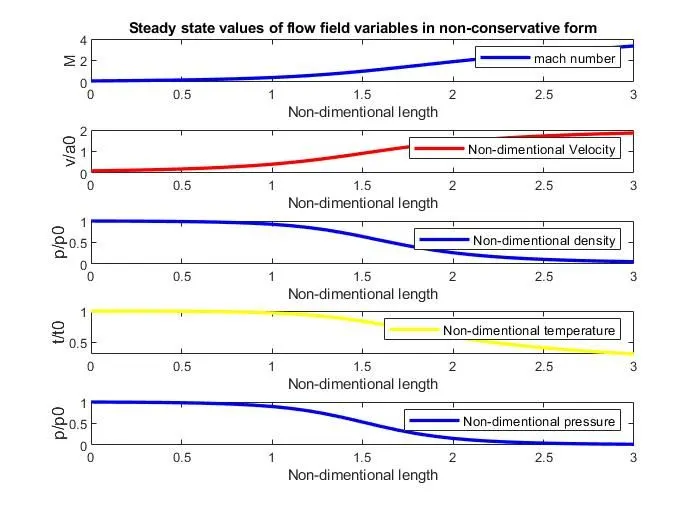
Results (Non-conservative forms of governing equations,n=31)
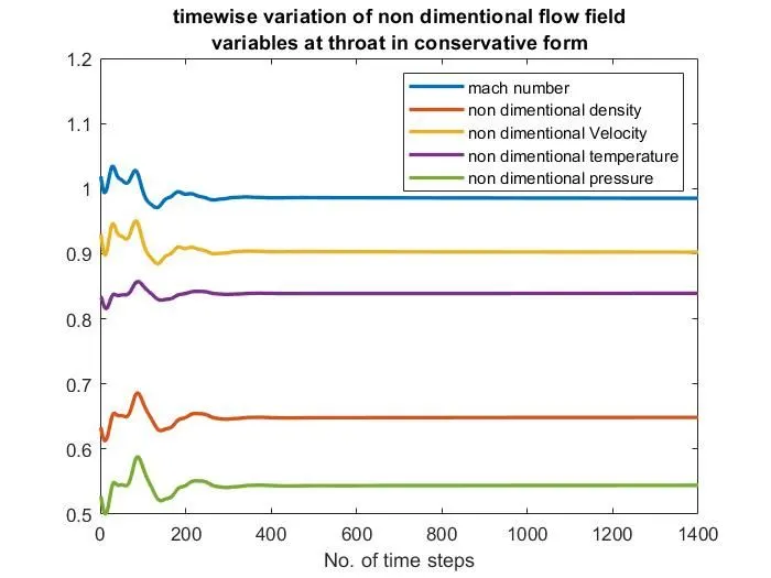
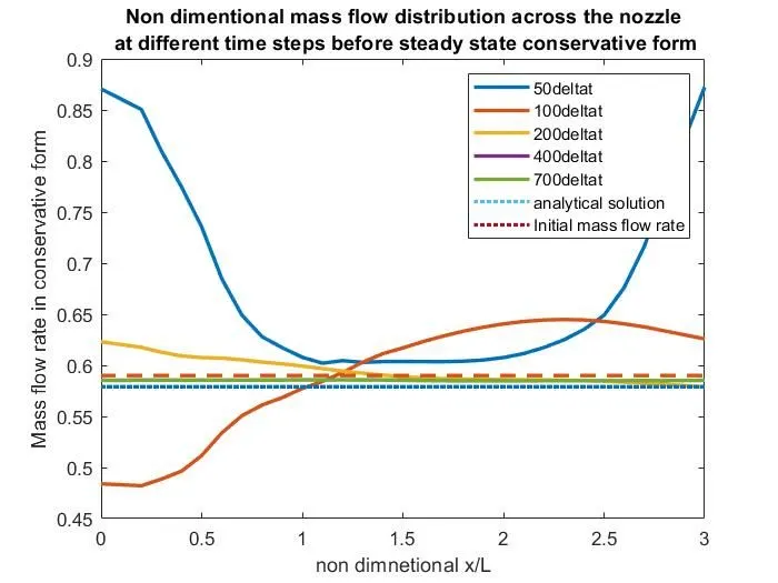
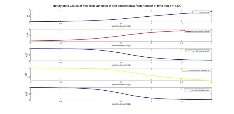
Results (Conservative forms of governing equations,n=31)
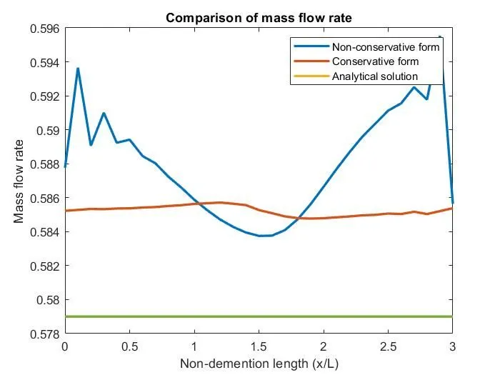
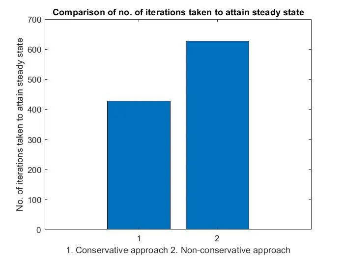
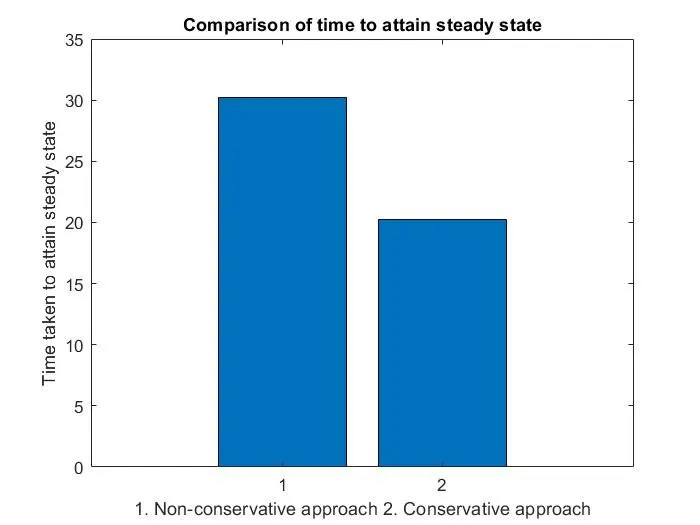
Comparison of mass flow rates
Grid independance test
|
Flow field variable (at throat section) |
M | `p/p_0` | `T/T_0` | `ρ/ρ_0` |
| Exact analytical solution | 1 | 0.528 | 0.833 | 0.639 |
| Non-conservative form (n=31) | 0.9994 | 0.5342 | 0.8365 | 0.6387 |
| Conservative form (n=31) | 0.9851 | 0.5442 | 0.8391 | 0.6486 |
| Non-conservative form (n=61) | 0.9997 | 0.5326 | 0.8354 | 0.6376 |
| Conservative form (n=61) | 0.9993 | 0.5330 | 0.8352 | 0.6382 |
Discussion and conclusion
- Mass flow distribution in conservative form is much closer to analytical value and it is somewhat constant. But in case of non-conservative case there is sizeable varation in mass flow distribution. This is because conservative from does better job of preserving mass throghout flow field.
- The non-conservation form leads to smaller residuals. Hence interms quality of algorithm, non-conservative from does better job.
- Both the forms of governing differential equations are satiffactory if we compare it with analytical solution.
- It takes around 500 time steps to get steady state solution.
- Variation of flow field variables are matching with the analytical results in both the cases.
- Solution is grid independent