Week 9 - FVM Literature Review
Aim: Study of finite volume method (FVM).
Theory:
In Computational Fluid Dynamics (CFD), governing equations of CFD are solved using numerical methods. In CFD partial differential equations (PDE) are first tranform into system of linear algebraic equations. The process of conversion of partial differential equations into system of linear algebaric equations in known as descritisation. There are two apprpaches of descritisation in CFD namely finite difference method (FDM) and finite volume method (FVM).
Finite difference method (FDM)
This method uses differential form of governing equations as a starting point. In this method derivatives in PDE's are replaced with finite difference that approxomates it. Accordingly it can be first order forward difference, first order backward difference, first order central difference, second order central difference etc. In FDM the governing PDE is descritised at several points, known as grid points. So domain is devided into number of grid points. Governing PDE's are coverted into system of linear algebraic equations and solved using sutaible numerical method.
Finite volume method (FVM)
This method uses integral form of governing equations as a starting point. In FVM governing PDE's are integrated over a entire controll volume and converted into system of linear algebraic equations. In FVM domain is devided into number of controll volumes. This process is called meshing. Then govening PDE is sloved at the center of controll volume and system of linear algebraic equations are obtained and and solved using sutaible numerical method.
Comparison between FDM and FVM
| Sr. no | FVM | FDM |
| 1 | Can be applied to unstructured mesh or grid | It can only be applied to structured or cartesian orthogonal grid. |
| 2 | Difficult to implement or difficult to code. | Easy to implement or easy to code. |
| 3 | It by default ensures the conservation of physical quantity. | It does not ensures the conservation of physical quantity. |
| 4 | Conceptually simple. | Conceptually difficult. |
| 5 | Computational domain is divided into finite number of controll volumes. | Computational domain is divided into finite number of grid points. |
| 6 | Suitable for complex geometries | Not suitable for complex geometries. |
Descritisation of 1D, steady, heat conduction equation without internal heat generation using FDM and FVM
a) FDM
Computational domain is as shown in figure
Governing differential equation is
`d/dx (k (dT)/dx)=0`
If K is constant then
`(d^2 T)/(dx^2) =0`
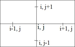
Figure: Computational domain
From central difference formula we can write,
`(d^2 T)/dx^2 =(T(i+1,j)−2T(i,j)+T(i-1,j))/(∆x)^2`
This is descritised from of governing equation at point (i,j). Likewise descritised form of governing equation is obtained at each point which results into system linear algebraic equations which can be solved using suitable numerical method to get T.
b) FVM
Governing differential equation is
`d/dx (k (dT)/dx)=0`
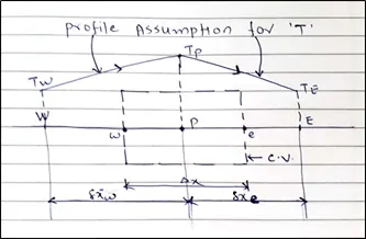
P is center of cell at which we need to find out T.
Rectangular part (--lines) is cell.
e and w represents west and east face of cell.
E and W represents cell centers on east and west sides.
Figure: Controll volume
Integrating over a controll volume
`∫_w^ed/dx (k (dT)/dx)=0`
`[k (dT)/dx]_e-[k (dT)/dx]_w=0`
Assuming peicewise linear varaition of T,
`k_e ((T_E-T_p)/(δx_e))-k_w ((T_p-T_w)/(δx_w ))=0`
Hence, `a_P T_P=a_E T_E+a_w T_w`
Above equation is descritised form of governing equation at point P. Likewise descritised form of governing equation is obtained at each point which results into system linear algebraic equations which can be solved using suitable numerical method to get T.
Where `a_E=k_e/(δx_e)`, `a_w=k_w/(δx_w)`and `a_P=a_E+a_w`
Interpolation schemes in CFD
Interpolation schemes are used for computation of a physical varaible in CFD. Some of the schemes are explain below.
1) Central difference scheme
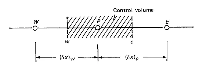
This scheme assumes that profile variation for varaible under consieration is linear between grid points. In this scheme value of varaible at e and w is calculated from following expression (for any general varaible ∅).
`∅_e= 1/2 (∅_E+∅_P )` and
`∅_w= 1/2 (∅_P+∅_W )`
This schemes fails when diffusion strength is very weak compared to convection strength or when cell peclet no. is more than 2.
2) The upwind scheme
According to this scheme,
`∅_e=∅_P`, if mass flow rate is along positive x-axis (left to right) and
`∅_e=∅_E`, if mass flow rate is along negative x-axis (right to left)
This scheme works even if cell peclet no. is more than 2. But it overpredicts diffusion.
3) Exponential scheme
In this scheme profile variation of ∅ between is asssumed to be exponential between grid points. Between points P and E, we can write,
`(∅-∅_P)/(∅_E-∅_P )=(e^(P_e (x/(δx)_e ) )-1)/(e^(P_e )-1)`
By integrating above equation over a controll volume and arranging it in the form of `a_P ∅_P=a_E ∅_E+a_w ∅_w`
we get
`a_P= [(F_e e^(P_e ))/(e^(p_e )-1)+F_e/(e^(p_w )-1)]`
`a_E=(F_e )/(e^(p_e )-1)`
`(F_w e^(P_w ))/(e^(p_w )-1)`
Where, `F= ρ u`= Convection strength
`P= F/D` = Cell peclet No.
Where, `D=γ/(δx)`
Where `γ` is diffusion coeficient
This scheme is ideal scheme as it is based on analytical solution. But it is not popular as it is computationally expensive.
4) Hybrid scheme
It is identical with central difference scheme for `-2≤P_e≤2` and outside this range it reduces to upwind scheme.
Flux limiters in CFD
It is used in numerical scehems to solved fluid dynamics problems which are govern by PDE's. They are used to avoid wiggles in the numerical solution due shocks, discontinuities or sharp changes in solution domain.