Week 3 - Taylor table method and Matlab code

Aim:

a) To derive 4th order approximations of the second-order derivative by using central scheme, right-sided scheme and left-sided scheme.

b) To compare the second order analytical derivative and second order derivative obtained by 4th order approximations (central scheme, right sided scheme and left-sided scheme) for a analytical function `e^xcosx`using MATLAB code.

Theory

In the finite difference method derivatives in the partial differential equations are replaced by the finite differences that approximates them. The accuracy of solution obtained is depends upon the equation to be solved and the numerical method used to obtained the solution. Higher the order of numerical approximation, higher is the accuracy of solution.

In the current work, expression of 2nd order derivative of a given function is found uisng taylors table method by using central scheme, right-sided scheme and left-sided scheme and it is proved that all schemes are 4th order accurate. Comaprison of second order analytical derivative and derivative obtained by numerical approximation is made using MATLAB code. It is shown that central scheme is more accurate compare to other two schemes.

Central scheme`

Here no. of nodes are taken using following equation,

The order of accuracy P = Number of nodes in the stencil N - order of derivative Q + 1

Hence no of nodes considered are 5.

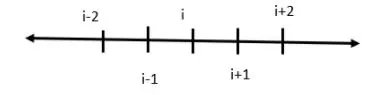
Hence equation for second order central difference is,

`(δ^2f)/(δx^2)`= a𝑓(𝑖-1)+b𝑓(𝑖-2)+c𝑓(𝑖)+𝑑𝑓(𝑖+1)+𝑒𝑓(𝑖+2)`

Now, the aim is to calculate coeficients a,b,c,d and e.

Taylors table for central scheme

	1	2	3	4	5	6	7
	f(i)	`∆x(∂f)/(∂x)`	`(∆x)^2 ((∂^2 f)/(∂x^2 ))`	`(∆x)^3 ((∂^3 f)/(∂x^3 ))`	`(∆x)^4 ((∂^4f)/(∂x^4 ))`	`(∆x)^5 ((∂^5 f)/(∂x^5 ))`	`(∆x)^6 ((∂^6 f)/(∂x^6 ))`
a f(i-2)	a	-2a	2a	-8a/6	16a/24	-32a/120	64a/720
b f(i-1)	b	-b	b/2	-b/6	b/24	-b/120	b/720
c f(i)	c	0	0	0	0	0	0
d f(i+1)	d	d	d/2	d/6	d/24	d/120	d/720
e f(i+2)	e	2e	2e	8e/6	16e/24	32e/120	64e/720
Total	0	0	1	0	0	Unknown	Unknown

Above table gives set of algebraic equations, as follows

`a+b+c+d+e=0;`

`-2a-b+0+d+2e=0;`

`2a+(b/2)+0+(d/2)+2e=1;`

`(-8a/6)-(b/6)+0+(d/6)+(8e/6)=0;`

`(16a/24)+(b/24)+0+(d/24)+(16e/24)=0`

By solving above equations by matrix inverion method using MATLAB, we get

a= -0.0833, b= 1.3333, c= -2.5, d=1.3333, e=-0.0833

Now from Taylors table `(∆x)^2 ((∂^2 f)/(∂x^2 ))``= a𝑓(𝑖-1)+b𝑓(𝑖-2)+c𝑓(𝑖)+𝑑𝑓(𝑖+1)+𝑒𝑓(𝑖+2)

Hence `((∂^2 f)/(∂x^2 )) = (af(i-1)+bf(i-2)+cf(i)+df(i+1)+ef(i+2))/(△x)^2`

In taylors table sum of column 1,2,4,5 and 6 (a=e and b=d) is zero and sum of column 3 is one (Being second order derivative). And some of column 6 and 7 is unkonwn.

Hence we can write

`((∂^2 f)/(∂x^2 ))=(∆x)^2 ((∂^2 f)/(∂x^2 )) (2a+b/2+0+d/2+2e)+(∆x)^6 ((∂^6 f)/(∂x^6 ))(64a/720+b/720+d/720+64e/720)+O(Δx)^7```

Also

`(∂^2 f)/(∂x^2 ) =a f(i-2)+b f(i-1)+c f(i)+d f(i+1)+e f(i+2)`

on deviding by `(Δx)^2` we get

`(∂^2 f)/(∂x^2 ) =(a f(i-2)+b f(i-1)+c f(i)+d f(i+1)+e f(i+2))/(Δx)^2 + O(Δx)^4`

Hence this scheme is 4th order accurate.

Skewed right-sided scheme

Here no. of nodes are taken using following equation,

The order of accuracy P = Number of nodes in the stencil N - order of derivative Q .

Hence no. of nodes considered are 6.

Hence equation for second order right-sided skewed sheme is,

`(δ^2f)/(δx^2)` =𝑎𝑓(𝑖)+𝑏𝑓(𝑖+1)+𝑐𝑓(𝑖+2)+𝑑𝑓(𝑖+3)+𝑒𝑓(𝑖+4)+g 𝑓(𝑖+5)

Now, the aim is to calculate coeficients a,b,c,d, e and g .

Taylors table for skewed right-sided scheme

	1	2	3	4	5	6	7
	f(i)	`∆x(∂f)/(∂x)`	`(∆x)^2 ((∂^2 f)/(∂x^2 ))`	`(∆x)^3 ((∂^3 f)/(∂x^3 ))`	`(∆x)^4 ((∂^4f)/(∂x^4 ))`	`(∆x)^5 ((∂^5 f)/(∂x^5 ))`	`(∆x)^6 ((∂^6 f)/(∂x^6 ))`
a f(i)	a	0	0	0	0	0	0
b f(i+1)	b	b	b/2	b/6	b/24	b/120	b/720
c f(i+2)	c	2c	2c	8c/6	16c/24	32c/120	64c/720
d f(i+3)	d	3d	9d/2	27d/6	81d/24	243d/120	729d/720
e f(i+4)	e	4e	8e	64d/6	256e/24	1024e/120	4096e/720
g f(i+5)	g	5g	25g/2	125g/6	625g/24	3125g/120	15625g/720
Total	0	0	1	0	0	0	Unknown

Above table gives set of algebraic equations, as follows

`a+b+c+d+e+g=0;`

`0+b+2c+3d+4e+5g=0`

`0+(b/2)+(2c)+(9d/2)+(8e)+(25/2g)`

`0+(b/6)+(8c/6)+(27d/6)+(64e/6)+(125/6g)`

`0+(b/24)+(16c/24)+(81d/24)+(256e/24)+(625/24g)`

`0+(b/120)+(32c/120)+(243d/120)+(1024e/120)+(3125/120g)`

By solving above equations by matrix inverion method using MATLAB, we get

a= 3.7500, b= -12.8333, c= 17.8333, d=-13.0000, e=5.0833, g=-0.8333

Now from Taylors table `(∆x)^2 ((∂^2 f)/(∂x^2 ))= f(i)+bf(i+1)+cf(i+2)+df(i+3)+ef(i+4)+g f(i+5)`

Hence `((∂^2 f)/(∂x^2 )) = (af(i)+bf(i+1)+cf(i+2)+df(i+3)+ef(i+4)+g f(i+5))/(△x)^2`

In taylors table sum of column 1,2,4,5 and 6 is zero and sum of column 3 is one (Being second order derivative). And some of column 7 is unkonwn.

Hence we can write

`((∂^2 f)/(∂x^2 ))=(∆x)^2 ((∂^2 f)/(∂x^2 )) (0+b/2+2c+9d/2+8e+25g/2)+(∆x)^6 ((∂^6 f)/(∂x^6 ))(0+b/720+64c/720+729d/720+4096e/720+15625g/720)```

Also

`(∂^2 f)/(∂x^2 ) =a f(i)+b f(i+1)+c f(i+2)+d f(i+3)+e f(i+4)+ g f(i+5)`

on deviding by `(Δx)^2` we get

`(∂^2 f)/(∂x^2 ) =(a f(i)+b f(i+1)+c f(i+2)+d f(i+3)+e f(i+4)+g f(i+5))/(Δx)^2 + O(Δx)^4`

Hence this scheme is 4th order accurate.

Taylors table for skewed left-sided scheme

Here no. of nodes are taken using following equation,

The order of accuracy P = Number of nodes in the stencil N - order of derivative Q .

Hence no. of nodes considered are 6.

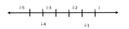
Now, the aim is to calculate coeficients a,b,c,d, e and g .

Taylors table

	1	2	3	4	5	6	7
	f(i)	`∆x(∂f)/(∂x)`	`(∆x)^2 ((∂^2 f)/(∂x^2 ))`	`(∆x)^3 ((∂^3 f)/(∂x^3 ))`	`(∆x)^4 ((∂^4f)/(∂x^4 ))`	`(∆x)^5 ((∂^5 f)/(∂x^5 ))`	`(∆x)^6 ((∂^6 f)/(∂x^6 ))`
a f(i)	a	0	0	0	0	0	0
b f(i+1)	b	-b	b/2	-b/6	b/24	-b/120	b/720
c f(i+2)	c	-2c	2c	-8c/6	16c/24	-32c/120	64c/720
d f(i+3)	d	-3d	9d/2	-27d/6	81d/24	-243d/120	729d/720
e f(i+4)	e	-4e	8e	-64d/6	256e/24	-1024e/120	4096e/720
g f(i+5)	f	-5f	25f/2	-125f/6	625f/24	-3125f/120	15625f/720
Total	0	0	1	0	0	0	Unknown

Above table gives set of algebraic equations, as follows

`a+b+c+d+e+g=0;`

`0-b-2c-3d-4e-5g=0`

`0+(b/2)+(2c)+(9d/2)+(8e)+(25/2g)`

`0-(b/6)-(8c/6)-(27d/6)-(64e/6)-(125/6g)`

`0+(b/24)+(16c/24)+(81d/24)+(256e/24)+(625/24g)`

`0-(b/120)-(32c/120)-(243d/120)-(1024e/120)-(3125/120g)`

a= 3.7500, b= -12.8333, c= 17.8333, d=-13.0000, e=5.0833, g=-0.8333

Now from Taylors table `(∆x)^2 ((∂^2 f)/(∂x^2 ))``= f(i)+bf(i-1)+cf(i-2)+df(i-3)+ef(i-4)+g f(i-5)

Hence `((∂^2 f)/(∂x^2 )) = (af(i)+bf(i+1)+cf(i+2)+df(i+3)+ef(i+4)+g f(i+5))/(△x)^2`

Here also similalry we can prove, this scheme is also 4th order accurate.

MATLAB CODE

% Central scheme
A = [1 1 1 1 1; -2 -1 0 1 2; 2 0.5 0 0.5 2; -8/6 -1/6 0 1/6 8/6; 16/24 1/24 0 1/24 16/24];
B = [0;0;1;0;0];
X = A\B;

Code is started with 'clear all', 'close all' and 'clc'.

clear all
close all
clc

Value of 'x' is defined at which, we have to compare the value of error for second order error in case of central scheme, Skewed right-sided difference and Skewed left-sided difference.

% To define value of x
x=pi/3;

Range of step size is defined.

% To defined range of step size
dx = linspace(pi/4, pi/400,20);

By suing taylors table coeficients are found out using matrix inversion method in MATLAB. X,Y and Z are arrays which containes values of coeficients of central, right-sided and left-sided scheme. A, B and C are coeficients matrices central, right-sided and left-sided scheme. And B, D and F are known column matrices of central, right-sided and left-sided scheme.

1. Central scheme

% Central scheme
A = [1 1 1 1 1; -2 -1 0 1 2; 2 0.5 0 0.5 2; -8/6 -1/6 0 1/6 8/6; 16/24 1/24 0 1/24 16/24];
B = [0;0;1;0;0];
X = A\B;

2. Skewed right-sided difference

% Right-sided skewed scheme
C = [1 1 1 1 1 1; 0 1 2 3 4 5; 0 1/2 2 9/2 8 25/2; 0 1/6 8/6 27/6 64/6 125/6; 0 1/24 16/24 81/24 256/24 625/24; 0 1/120 32/120 243/120 1024/120 3125/120];
D = [0;0;1;0;0;0];
Y = C\D;

3. Skewed left-sided difference

% Left-sided skewed scheme
E  = [1 1 1 1 1 1; 0 -1 -2 -3 -4 -5; 0 1/2 2 9/2 8 25/2; 0 -1/6 -8/6 -27/6 -64/6 -125/6; 0 1/24 16/24 81/24 256/24 625/24; 0 -1/120 -32/120 -243/120 -1024/120 -3125/120];
F = [0;0;1;0;0;0];
Z = E\F;

Function codes are called for central, right-sided and left-sided scheme. For loop is uded from i=1 to length(dx) to calculate error in all three schemes.

% Calculation of error for Central, right-sided and left-sided skewed
% scheme by calling function
for i = 1:length(dx)
    Central_differencing_approximation_error(i) = central(x,dx(i),X);
    Right_side_skewed_approximation_error(i) = right_side_skewed(x,dx(i),Y);
    Left_side_skewed_approximation_error(i) = left_side_skewed(x,dx(i),Z);
end

Function codes are explained below. In all fucntion codes, first analytical derivative of a given function is calculated. Then numerical derivative is calculated. After error is absolue error is calculated as difference between two derivatives obtained.

% Function code to calculate absolute error between analytical and
% Numerical derivative for central scheme
function out1 = central(x,dx,X)
analytical_derivative = (-2*exp(x)*sin(x));
Central_differencing_approximation = (X(1)*fof(x-2*dx)+X(2)*fof(x-dx)+X(3)*fof(x)+X(4)*fof(x+dx)+X(5)*fof(x+2*dx))/(dx^2);
out1 = abs(Central_differencing_approximation - analytical_derivative);
end

% Function code to calculate absolute error between analytical and
% Numerical derivative for left-sided skewed scheme
function out3 = left_side_skewed(x,dx,Z)
analytical_derivative = (-2*exp(x)*sin(x));
Left_side_skewed_approximation = (Z(1)*fof(x)+Z(2)*fof(x-dx)+Z(3)*fof(x-2*dx)+Z(4)*fof(x-3*dx)+Z(5)*fof(x-4*dx)+Z(6)*fof(x-5*dx))/(dx^2);
out3 = abs(Left_side_skewed_approximation - analytical_derivative);
end

% Function code to calculate absolute error between analytical and
% Numerical derivative for right-sided skewed scheme
function out2 = right_side_skewed(x,dx,Y)
analytical_derivative = (-2*exp(x)*sin(x));
Right_side_skewed_approximation = (Y(1)*fof(x)+Y(2)*fof(x+dx)+Y(3)*fof(x+2*dx)+Y(4)*fof(x+3*dx)+Y(5)*fof(x+4*dx)+Y(6)*fof(x+5*dx))/(dx^2);
out2 = abs(Right_side_skewed_approximation - analytical_derivative);
end

saperate function code is written to calculate Numerical derivative to avoid writing of long exoressions.

function y = fof(x)
y = exp(x)*cos(x);
end

Variation of error with respect to step size is plotted for all three schemes. Legends are given to plot using 'legend command' and labels are iven to x and y axis using 'xlabel' and 'ylabel' command.

figure(1)
loglog(dx,Central_differencing_approximation_error, 'color','r', 'marker','o')
hold on
loglog(dx,Right_side_skewed_approximation_error, 'color','b', 'marker','o')
loglog(dx, Left_side_skewed_approximation_error, 'color','g', 'marker','o')
legend('Central differencing approximation error','Right side skewed approximation error','Left side skewed approximation error')
xlabel('Step size')
ylabel('Absolute error')

Complete code

% MATLAB code to calcualte abolute error for 4th order accurate schemes.
clear all
close all
clc

% To define value of x
x=pi/3;

% To defined range of step size
dx = linspace(pi/4, pi/400,20);

% Central scheme
A = [1 1 1 1 1; -2 -1 0 1 2; 2 0.5 0 0.5 2; -8/6 -1/6 0 1/6 8/6; 16/24 1/24 0 1/24 16/24];
B = [0;0;1;0;0];
X = A\B;

% Right-sided skewed scheme
C = [1 1 1 1 1 1; 0 1 2 3 4 5; 0 1/2 2 9/2 8 25/2; 0 1/6 8/6 27/6 64/6 125/6; 0 1/24 16/24 81/24 256/24 625/24; 0 1/120 32/120 243/120 1024/120 3125/120];
D = [0;0;1;0;0;0];
Y = C\D;

% Left-sided skewed scheme
E  = [1 1 1 1 1 1; 0 -1 -2 -3 -4 -5; 0 1/2 2 9/2 8 25/2; 0 -1/6 -8/6 -27/6 -64/6 -125/6; 0 1/24 16/24 81/24 256/24 625/24; 0 -1/120 -32/120 -243/120 -1024/120 -3125/120];
F = [0;0;1;0;0;0];
Z = E\F;

% Calculation of error for Central, right-sided and left-sided skewed
% scheme by calling function
for i = 1:length(dx)
    Central_differencing_approximation_error(i) = central(x,dx(i),X);
    Right_side_skewed_approximation_error(i) = right_side_skewed(x,dx(i),Y);
    Left_side_skewed_approximation_error(i) = left_side_skewed(x,dx(i),Z);
end

% Plotting of absolute error Vs step size
figure(1)
loglog(dx,Central_differencing_approximation_error, 'color','r', 'marker','o')
hold on
loglog(dx,Right_side_skewed_approximation_error, 'color','b', 'marker','o')
loglog(dx, Left_side_skewed_approximation_error, 'color','g', 'marker','o')
legend('Central differencing approximation error','Right side skewed approximation error','Left side skewed approximation error')
xlabel('Step size')
ylabel('Absolute error')
title({'Comparison of error for central scheme,right-sided'; 'skewed scheme, and left-sided skewed scheme'}, 'color','b')

Results

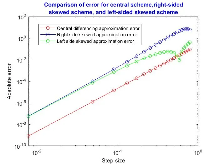
From above plot it is clear that central scheme is more accuate comapred to right-sided and left-sided skewed sheme. Also in all three schemes, as step size increses, absolute error also increases.