Week 1: Channel flow simulation using CONVERGE CFD
Title: Channel flow simulation using CONVERGE CFD.
Aim:
- Set up the case and to run the simulation for 3 dfferent mesh sizes and compare the results.
- Plot velocity contours and pressure contours for all 3 cases.
- To create velocity animation showing developed flow.
Theory:
In Engineering fluid flow may be an internal flow or external flow. Flow through close crossections like pipe is called internal flow. And flow over a surface, for example, flow over a flat plate is a example of external flow.
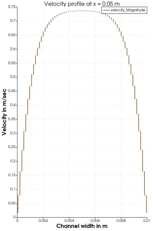
Internal flows are of extreame importance in engineering. In current project, flow through a channel of square cross-section is smulated. Pressure and velocity ditribution is studied. For an internal flow, velocity distribution is parabolic (zero at surface and maximum at center) as shown in diagram below.
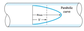
Fig: Velocity profile for internal flow
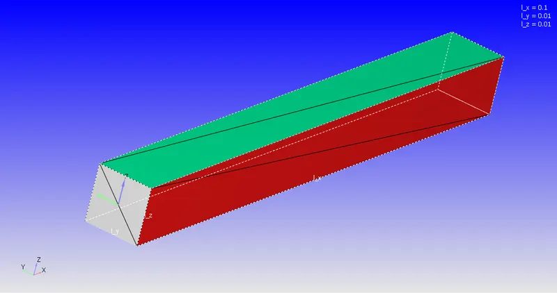
Geometry of computational domain
Dimentions of a model are 0.1 m, 0.01m and 0.01 m along x, y and z directions respectively.
Set up:
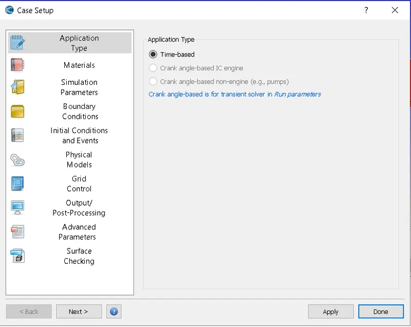
1) Application type
As it is problem which dont involves IC engine or pumps, time-based option is selected.
2) Materials
As working fluid is air, in predefined mixtures, air is selected, with species tab enabled.
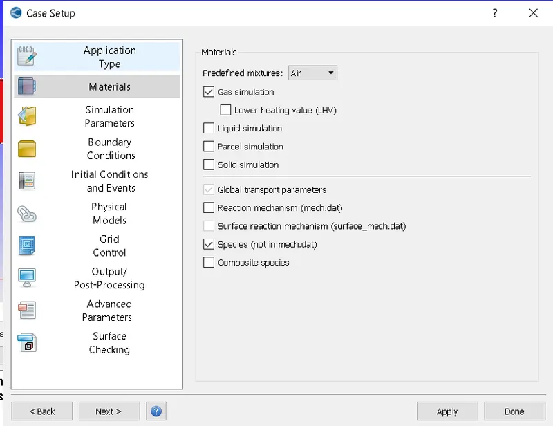
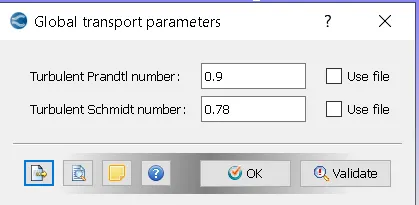
Global transport properties are kept default.
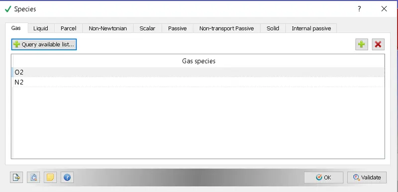
Species selected are O2 and N2
3) Simulation Parameters
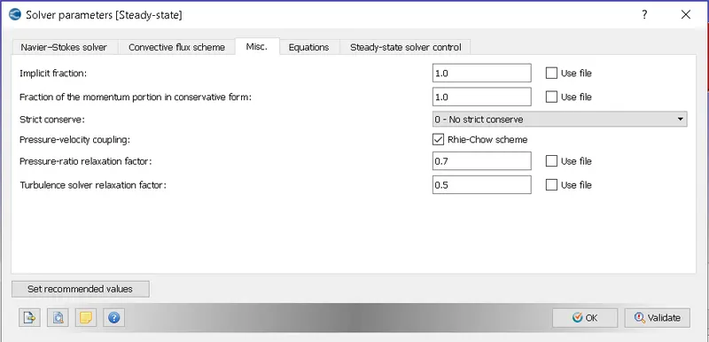
Steady state solver is selected, with full hydrodynamic simulation mode and compressible gas flow solver.
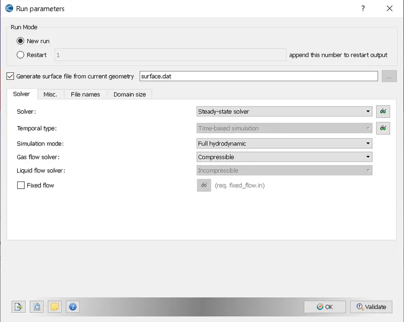
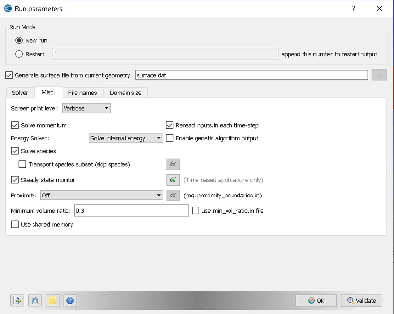
Here, steady state solver is ticked and and use shared memory is unticked.
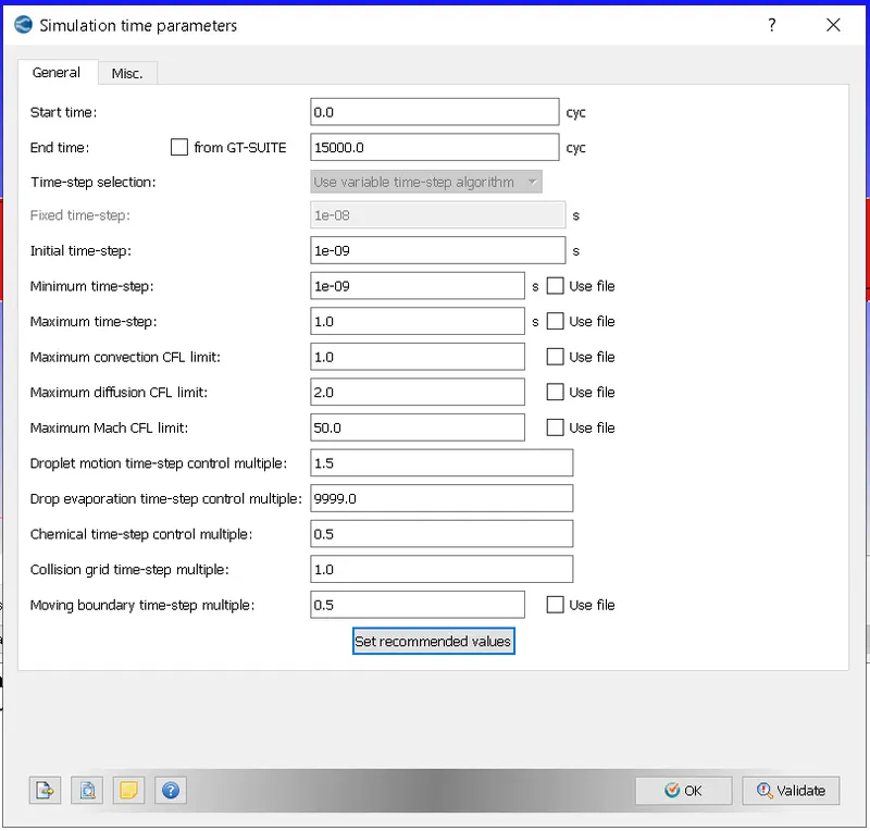
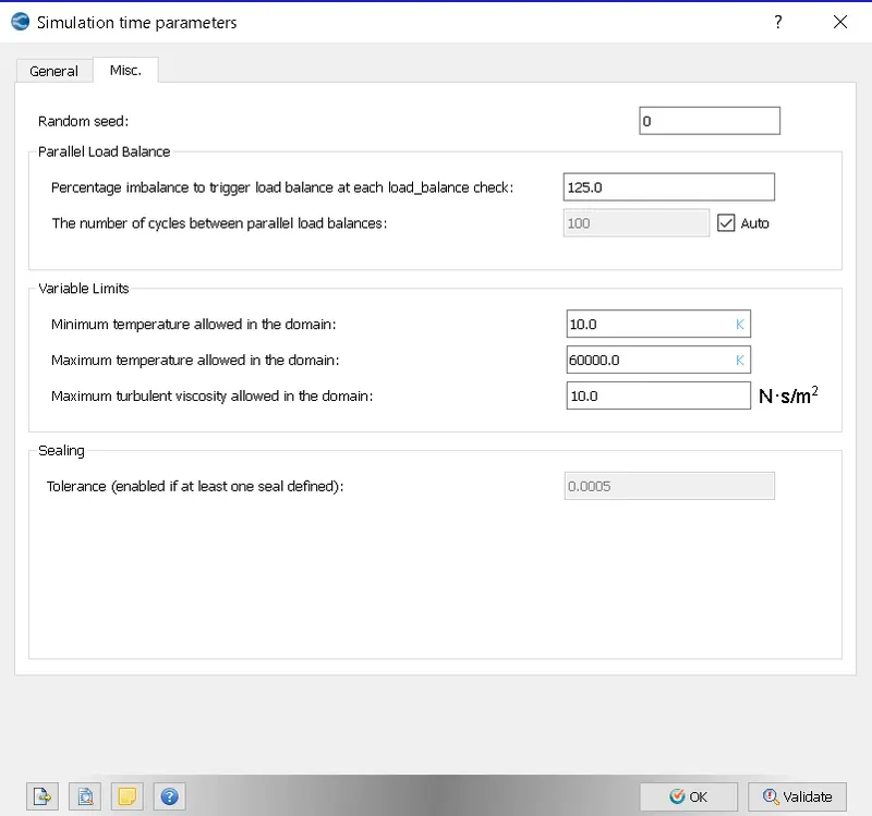
Start time = 0 cycles, end time is 15000 cycles, initial and minimum time step size = 1e-09, maximum time step size = 1, maximum conection CFL limit = 1.
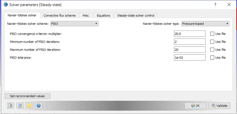
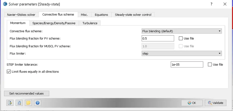
Here pressure based solver is selected, with PISO scheme.
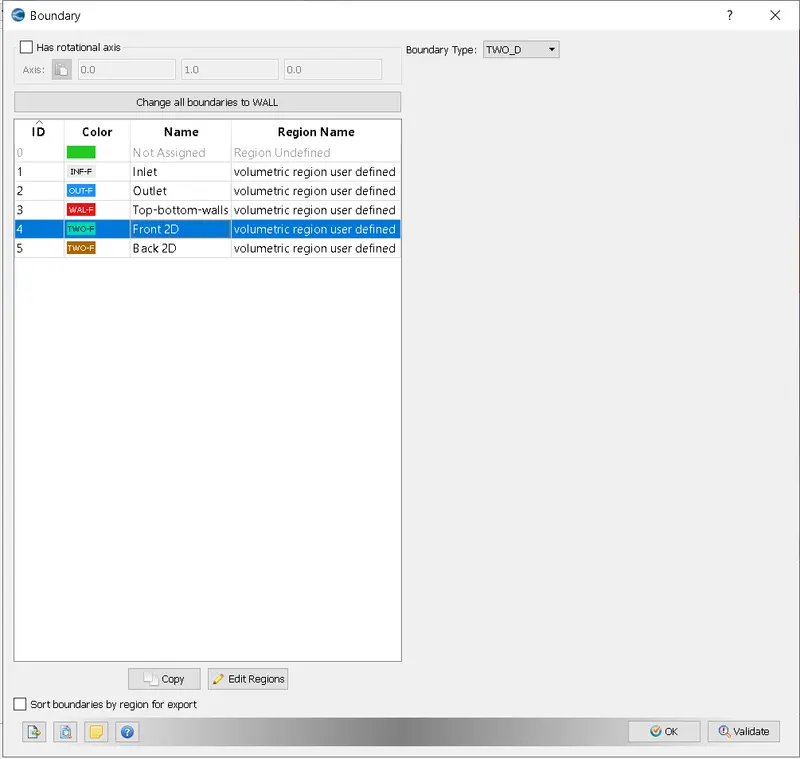
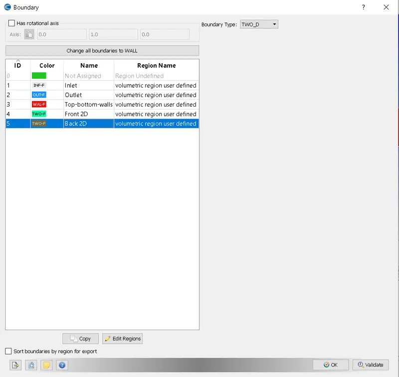
4) Boundary conditions
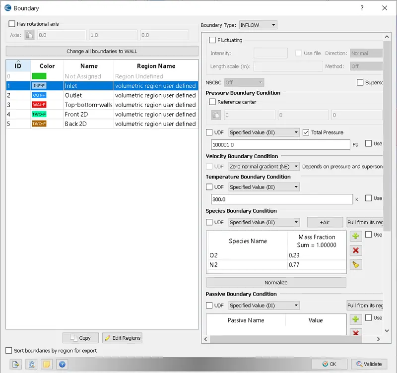
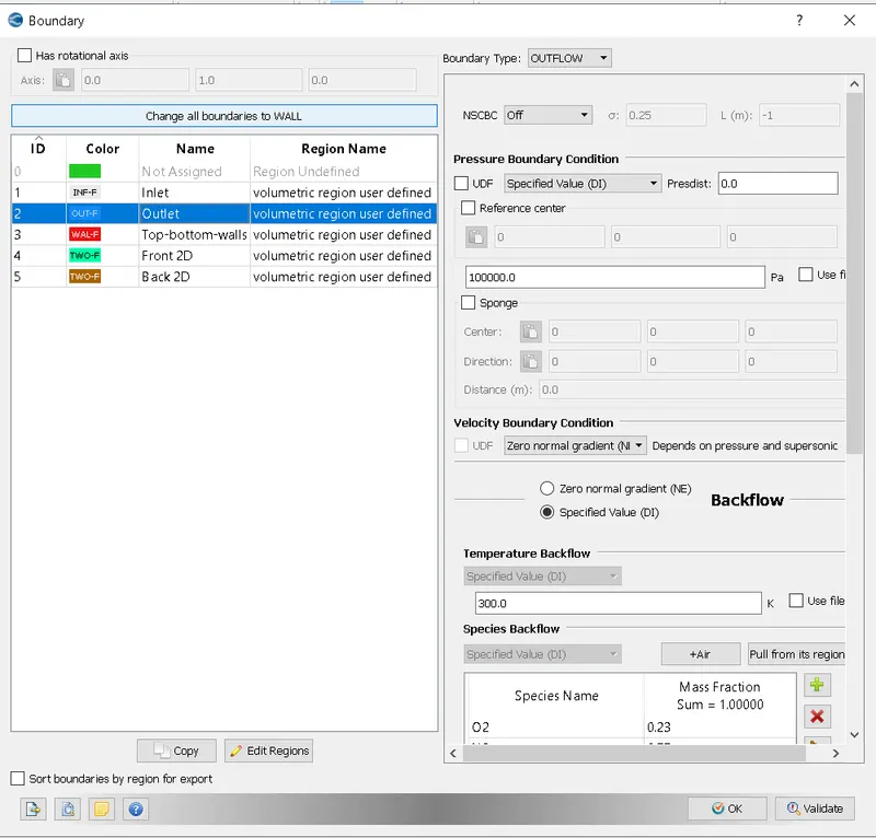
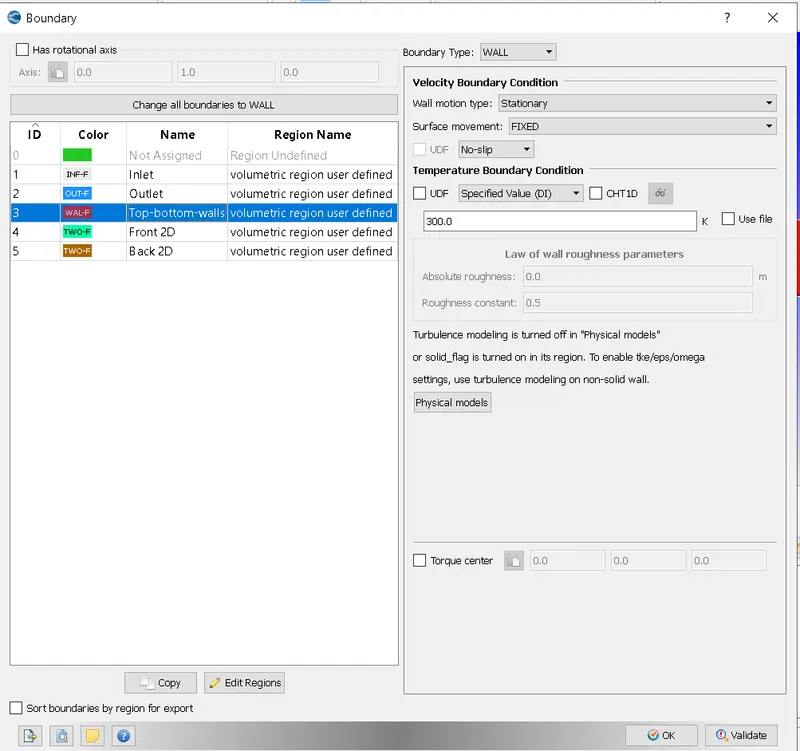
Following boundary conditions are provided
Inlet: Inflow
Outlet: Outflow
Top and bottom walls: Wall
Front and back 2D walls: Front 2D and back 2D respectively
5) Regions and Initialisation
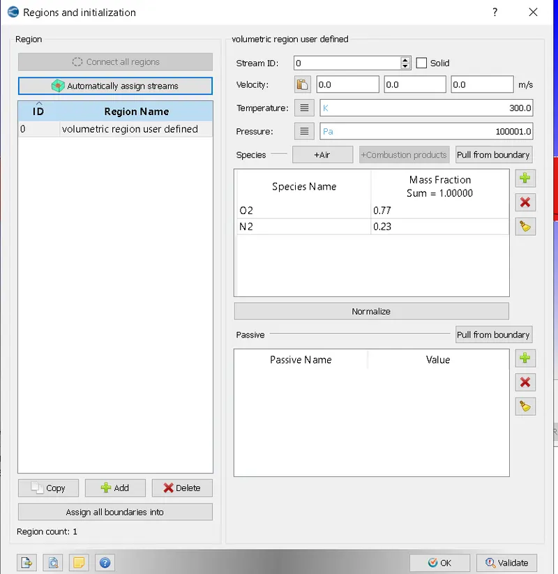
Initial velcoty= 0 m/sec
Initial Temp. = 300 K
Initial Pressure = 100001.0 Pa
6) Physical models
Here turbulance model is not enabled
7) Grid controll
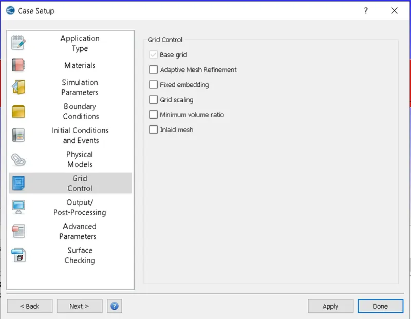
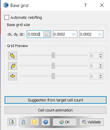
As shown 3 types of grids are taken for simulation with mesh size as 2e-4, 1.5e-4 and 1.2e-4.
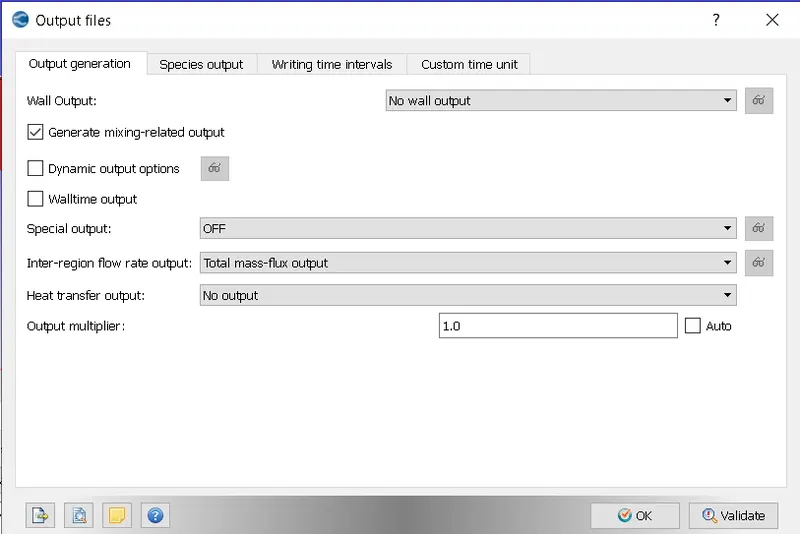
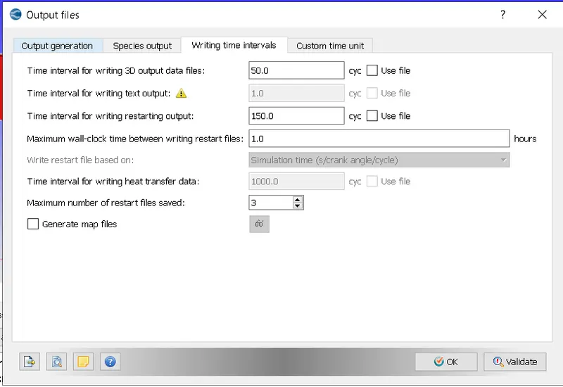
8) Output/Post processing
Results:
a) Mesh size 2e-4 m
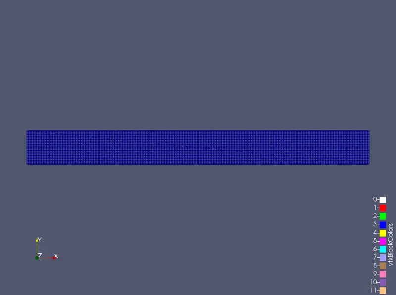
Mesh

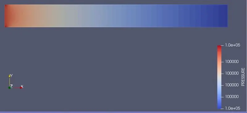
Pressure contour
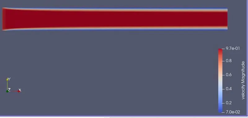
Velocity contour
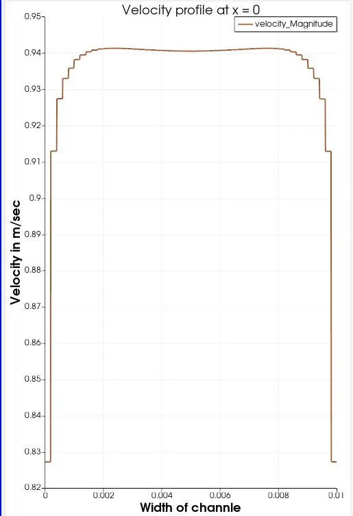
Velocity profile at x =0 m
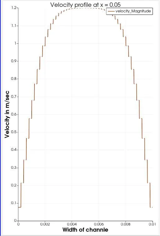
Velocity profile at x =0.05 m
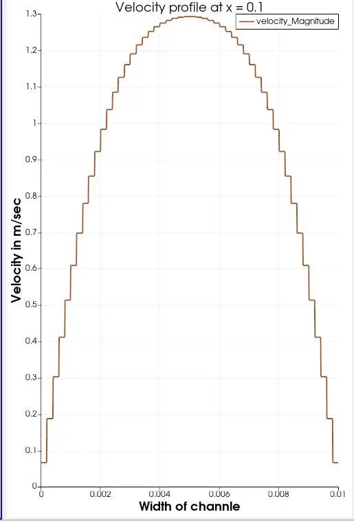
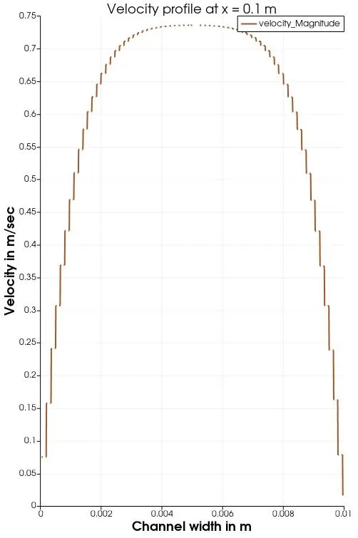
Velocity profile at x =0.1 m
Velocity animation: https://youtu.be/XJiCZ8qQBH8
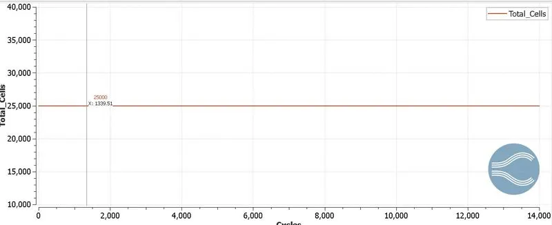
Total cell
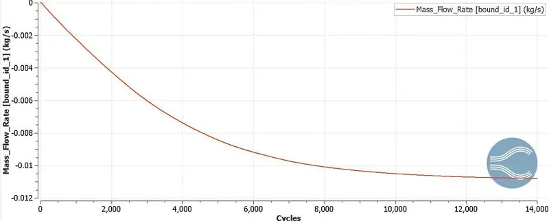
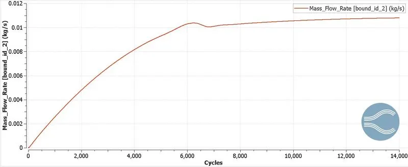
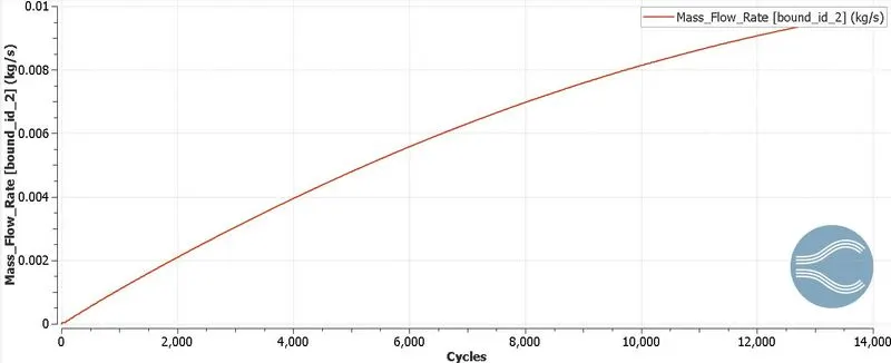
mass flow rate
b) Mesh size1.5e-4 m
Mesh
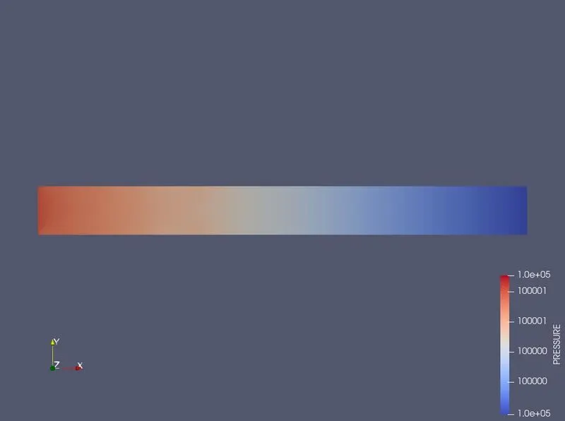
Pressure contour
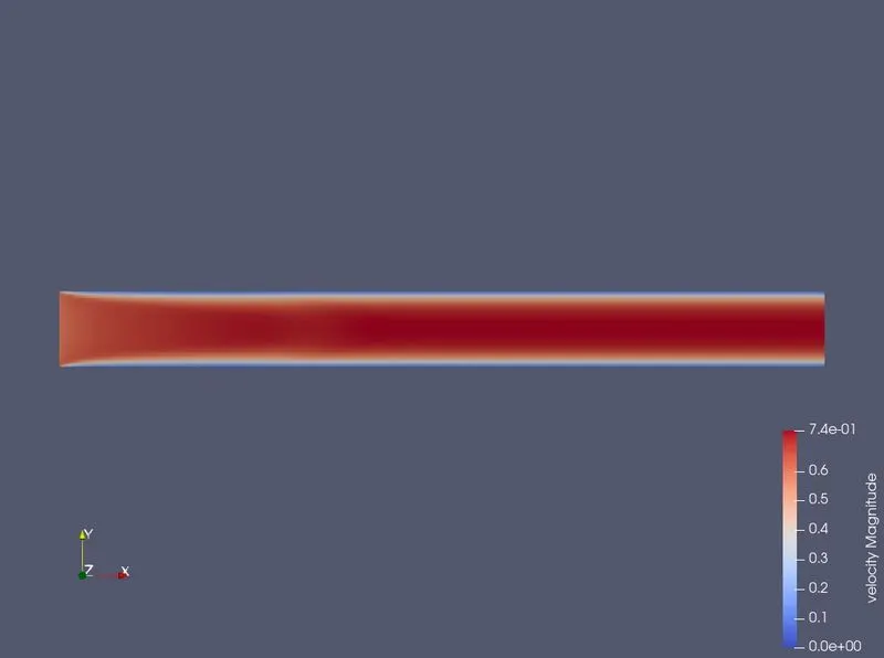
Velocity contour
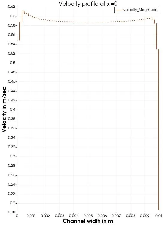
Velocity profile at x =0 m
Velocity profile at x =0.05 m
Velocity profile at x =0.1 m
Velocity animation : https://youtu.be/hbMilpojVEo
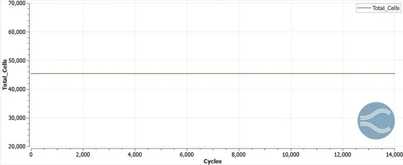
Total cell
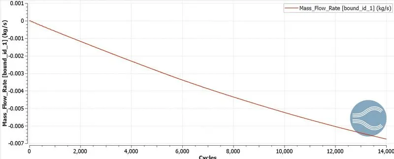
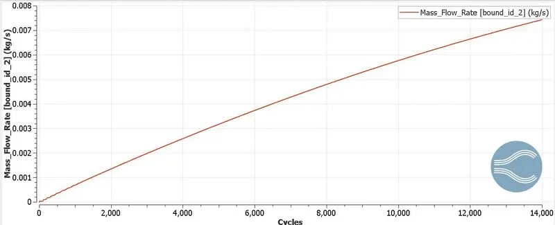
mass flow rate
c) Mesh size 1.2e-4 m
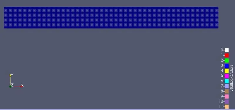
Mesh
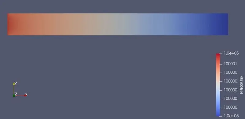
Pressure contour
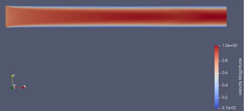
Velocity contour
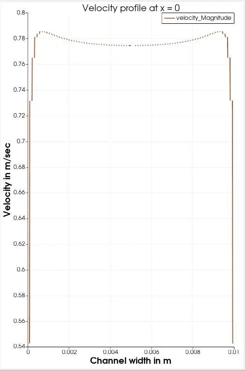
Velocity profile at x =0 m
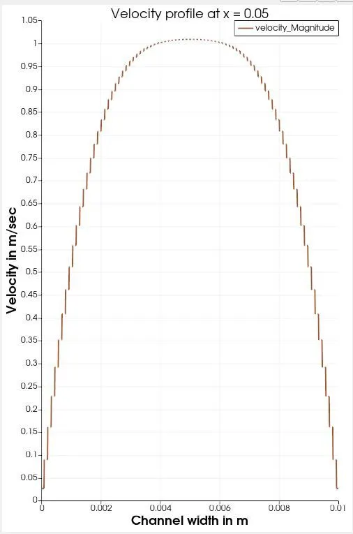
Velocity profile at x =0.05 m
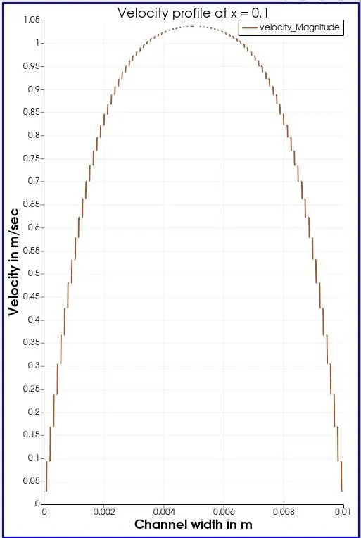
Velocity profile at x =0.1 m
Velocity animation : https://youtu.be/I317-AGLKj0
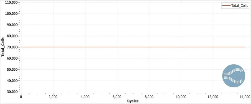
Total cell
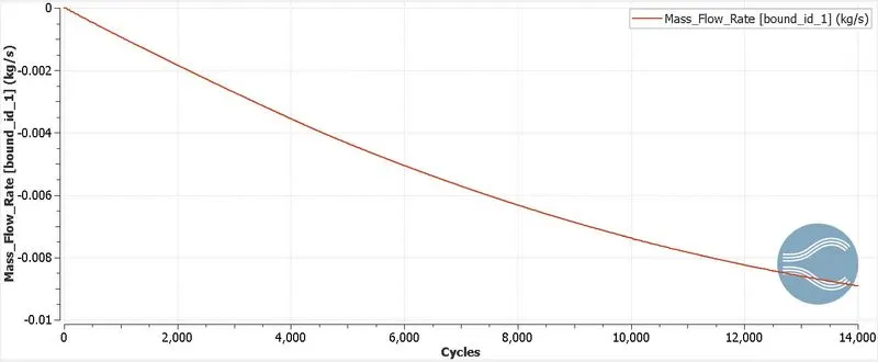
mass flow rate
Results and discussion
- Is it found that, with reduction in mesh size, computation time increases drastically.
- Velocity profile is found to be changing along length till certain value of x. Then velocity profile is found be contant with length.
- Pressure is decreasing along length.