Week 5 - Mid term project - Solving the steady and unsteady 2D heat conduction problem
Aim: To solve 2 dimensional (2D), steady and unsteady heat conduction equation using MATLAB.
Theory:
General heat conduction equation in Cartesian coordinates is given by
`(∂^2 T)/(∂x^2) +(∂^2 T)/(∂y^2) +(∂^2 T)/(∂z^2) =1/α (∂T)/(∂t)`
Where T is temperature, t is time and `α`is thermal diffusivity.
Now, 2D steady heat conduction equation is given by
`(∂^2 T)/(∂x^2)+(∂^2 T)/(∂y^2) =0` and
2D unsteady heat conduction equation is given by,
`(∂^2 T)/(∂x^2) +(∂^2 T)/(∂y^2) =1/α (∂T)/(∂t)`
In the current work 2D heat conduction equation is solved by using iterative techniques using MATLAB. Three iterative techniques are used namely Jacoby method, Gauss-Seidal method and successive over-relaxation method. Again unsteady heat conduction equation is solved using explicit and implicit methods.
In Jacobi method, to calculate temperature at current time step, all values are taken from privious time steps.
In Gauss-Seidel method, to calculate temperature at current time step, values are taken from privious as well as current time step.
In successive over-relxation method temperature is calculated from following expression
T = (1-w)Told + w Tj or T = (1-w)Told + w Tgs
Where w = relxation factor, Tj temperature by jacobi method and Tgs is temperature by Gauss-Seidel method.
Problem definition
A square domain is assumed with dimensions of 1 unit by 1 unit.
Following boundary conditions are used
Top Boundary = 600 K
Bottom Boundary = 900 K
Left Boundary = 400 K
Right Boundary = 800 K
Discretisation of heat conduction equation
a) 2D steady heat conduction equation
`(∂^2 T)/(∂x^2)+(∂^2 T)/(∂y^2) =0`
Let i and j be index in x and y directions respectively and `∆x`and `∆y`be grid spacing in x and y directions respectively.
By using finite difference method, above equation can be written as,
`(T_((i-1,j))-2T_(i.j)+T_((i+1,j)))/(∆x)^2 +(T_((i,j-1))-2T_((i,j))+T_((i,j+1)))/(∆y)^2 =0`
Hence,
`(T_L-2T_p+T_R)/(∆x)^2 +(T_B-2T_P+T_T)/(∆y)^2 =0`
Here Tp is point at which we have to solve above equation and TL, TR, TT, TB are the point on left side, right side, top side and bottom side of point P respectively.
On simplifying above equation,
`T_p= 1/k [(T_L+T_R)/(∆x)^2 +(T_T+T_B)/(∆y)^2 ]`
Above equation is descritized form of 2D steady heat conduction equation.
where
`=2((∆x)^2+(∆y)^2)/((∆x)^2 (∆y)^2 )`
a) 2D unsteady heat conduction equation
Explicite method
`(∂^2 T)/(∂x^2) +(∂^2 T)/(∂y^2) =1/α (∂T)/(∂t)`
`α((∂^2 T)/(∂x^2) +(∂^2 T)/(∂y^2)) = (∂T)/(∂t)`
By using finite difference method, above equation can be written as,
`(T_p^(n+1)-T_p^n)/(∆t)=α[(T_L^n-2T_p^n+T_R^n)/(∆x)^2 +(T_B^n-2T_P^n+T_T)^n/(∆y)^2 ]`
n denotes privious time step and (n+1) denotes current time step.
In explicite method to calculate variable at current time step, values are taken from privious time step only.
Therefore
`T_p^(n+1)= T_p^n+k_1 (T_L^n-2T_p^n+T_R^n )+k_2 (T_B^n-2T_P^n+T_T ^n)`
Above equation is descritized form of 2D unsteady heat conduction equation by explicit method.
Where
`k_1= (α.∆t)/(∆x)^2` and `k_2= (α.∆t)/(∆y)^2`
K1 and k2 are known as Courant–Friedrichs–Lewy number along x and y directions respectively.
For stability of a solution `k1+k2 ≤0.5`
Implicite method
In explicite method to calculate variable at current time step, values are taken from privious time step as well from current time steps.
Therefore
`(T_p^(n+1)-T_p^n)/(∆t)=α[(T_L^(n+1)-2T_p^(n+1)+T_R^(n+1))/(∆x)^2 +(T_B^(n+1)-2T_P^(n+1)+T_T)^(n+1)/(∆y)^2 ]`
On simplifying it, we get
`T_p^(n+1)= 1/((1+2k_1+2k_2 ) ) [T_p^n+k_1 (T_L^(n+1)+T_R^(n+1))+k_2 (T_T^(n+1)+T_B^(n+1))]`
Above equation is descritized form of 2D unsteady heat conduction equation by implicit method.
Where
MATLAB Code
Two space (for) loops are used to calculate temperatures.
Temperarures are calculated as long as error is greater that tolerence value.
Once error is less than tolerence values, code will come out of while loop and it will plot the results.
Results are plotted using contour plots.
1) Steady state
% Code to solve 2D steady heat conduction equation

clear all
close all
clc

% Inputs
nx=50; % No. of grid points x direction
ny=50; % No. of grid points y direction
L=1;   % Length of domain along x and y direction

x=linspace(0,L,nx); % To create x array
y=linspace(0,L,ny); % To create y array

dx=x(2)-x(1); % Grid spacing along x
dy=y(2)-y(1); % Grid spacing along y
w=1.1;        % Over-relaxation factor

% Initial condition at inner nodes of a domain
T = 300*ones(nx,ny);

%Boundary conditions
T(1,:)=600;
T(end,:)=900;
T(:,1)=400;
T(:,end)=800;

% Initial condition for Told temperature
Told=T;

% To calculate constant k2
k=2*((dx^2+dx^2)/(dx^2*dy^2));

% Temperature at 4 corners of doamin
T(1,1)= (600+400)/2;
T(1,end)= (600+800)/2;
T(end,1) = (400+900)/2;
T(end,end)=(800+900)/2;

% Tolerence value to compute error
tol=1e-4;

% Initialisation of error
error=9e9;

iterative_solvers = 1;

% Jacobi Method
tic
  jacobi_iter = 1;
  if iterative_solvers==1
    while(error>tol)
       for i=2:nx-1
          for j=2:ny-1
            m = (Told(i+1,j)+Told(i-1,j))/(dx^2);
            n = (Told(i,j+1)+Told(i,j-1))/(dy^2);
            T(i,j)=(m+n)/k;
          end
       end
    error = max(max(abs(Told-T)));
    Told=T;
    jacobi_iter=jacobi_iter+1;
    end

  time1=toc;
  figure(1);
  contourf(x,y,T,'ShowText', 'on')
  colorbar
  set(gca, 'YDIR', 'reverse')
  xlabel('X axis')
  ylabel('Temperature,T')
  title_text = sprintf('Iteration number = %d\nSimulation time=%d s',jacobi_iter, time1);
  title({'Jacobi method'; title_text})
  pause(0.03)
  end

% Gauss seidal Method
 tic
  gs_iter = 1;
  if iterative_solvers==2
    while(error>tol)
       for i=2:nx-1
          for j=2:ny-1
            m = (Told(i+1,j)+T(i-1,j))/(dx^2);
            n = (Told(i,j+1)+T(i,j-1))/(dy^2);
            T(i,j)=(m+n)/k;
          end
       end
    error = max(max(abs(Told-T)));
    Told=T;
    gs_iter=gs_iter+1;
    end

  time2=toc;
  figure(1);
  contourf(x,y,T,'ShowText', 'on')
  colorbar
  set(gca, 'YDIR', 'reverse')
  xlabel('X axis')
  ylabel('Temperature,T')
  title_text = sprintf('Iteration number = %d\nSimulation time=%d s',gs_iter, time2);
  title({'Gauss seidal method'; title_text})
  pause(0.03)
 end

% Sucessive over relaxation method
tic
  sor_iter = 1;
  if iterative_solvers==3
    while(error>tol)
       for i=2:nx-1
          for j=2:ny-1
            m = (Told(i+1,j)+T(i-1,j))/(dx^2);
            n = (Told(i,j+1)+T(i,j-1))/(dy^2);
            T(i,j)=(1-w)*Told(i,j)+w*((m+n)/k);
          end
       end
    error = max(max(abs(Told-T)));
    Told=T;
    sor_iter=sor_iter+1;
    end

  time3=toc;
  figure(1);
  contourf(x,y,T,'ShowText', 'on')
  colorbar
  set(gca, 'YDIR', 'reverse')
  xlabel('X axis')
  ylabel('Temperature,T')
  title_text = sprintf('Iteration number = %d\nSimulation time=%d s',sor_iter, time3);
  title({'Sucessive over relaxation method'; title_text})
  pause(0.03)
 end
2) Unsteady state
In unsteady case also same logic is used. In addition to, two space loops, one time loop is used as it is usntedy situation.
Results are plotted using contour plots.
a) Explicit method
% Code to solve 2D unsteady heat conduction equation using explicit method

clear all
close all
clc

% Inputs
nx=50;  % No. of grid points x direction
ny=50;  % No. of grid points y direction
L=1;   % Length of domain along x and y direction

x=linspace(0,L,nx); % To create x array
y=linspace(0,L,ny); % To create y array

dx=x(2)-x(1);  % Grid spacing along x
dy=y(2)-y(1);  % Grid spacing along y
w=1.1;         % Over-relaxation factor

dt=0.00001;   % Time step size
TT=0.4;       % Total simulation time
nt=TT/dt;     % No of time steps
alpha=1.4;    % Thermal diffusivity

CNx = (alpha*dt)/dx^2;  % CFL no along x
CNy = (alpha*dt)/dy^2;  % CFL no along y

% Initial conditions
T = 300*ones(nx,ny);

%Boundary conditions
T(1,:)=600;
T(end,:)=900;
T(:,1)=400;
T(:,end)=800;

% Calculation of CFL along x and y directions
k1 =(alpha*dt)/(dx^2);
k2 = (alpha*dt)/(dy^2);

% Temperature at 4 corners of doamin
T(1,1)= (600+400)/2;
T(1,end)= (600+800)/2;
T(end,1) = (400+900)/2;
T(end,end)=(800+900)/2;

% Initial condition for Told
Told=T;

% Initialisation of error
error = 9e9;

% Tolerence value to compute error
tol=1e-4;

iterative_solvers = 1;

% Jacobi Method
jacobi_iter = 1;
tic
if iterative_solvers==1
  for m=1:nt
    while(error>tol)
    for i=2:nx-1
        for j=2:ny-1
            term1=k1*(Told(i-1,j)-2*Told(i,j)+Told(i+1,j));
            term2=k2*(Told(i,j-1)-2*Told(i,j)+Told(i,j+1));
            T(i,j)=Told(i,j)+term1+term2;
        end
    end
    error = max(max(abs(Told-T)));
    Told=T;
    jacobi_iter=jacobi_iter+1;
    end
  end

  time1=toc;
  figure(1);
  contourf(x,y,T,'ShowText', 'on')
  colorbar
  set(gca, 'YDIR', 'reverse')
  xlabel('X axis')
  ylabel('Temperature,T')
  title_text = sprintf('Iteration number = %d\nSimulation time=%d s',jacobi_iter, time1);
  title({'Jacobi method'; title_text})
  pause(0.03)
end

% GS Method
tic
gs_iter = 1;
 if iterative_solvers==2
  for m=1:nt
    while(error>tol)
    for i=2:nx-1
        for j=2:ny-1
            term1=k1*(T(i-1,j)-2*T(i,j)+Told(i+1,j));
            term2=k2*(T(i,j-1)-2*T(i,j)+Told(i,j+1));
            T(i,j)=Told(i,j)+term1+term2;
        end
    end
    error = max(max(abs(Told-T)));
    Told=T;
    gs_iter=gs_iter+1;
    end
  end

  time2=toc;
  figure(1);
  contourf(x,y,T,'ShowText', 'on')
  colorbar
  set(gca, 'YDIR', 'reverse')
  xlabel('X axis')
  ylabel('Temperature,T')
  title_text = sprintf('Iteration number = %d\nSimulation time=%d s',gs_iter, time2);
  title({'Gauss seidal method'; title_text})
  pause(0.03)
 end

% SOR Method
tic
sor_iter = 1;
 if iterative_solvers==3
  for m=1:nt
    while(error>tol)
    for i=2:nx-1
        for j=2:ny-1
            term1=k1*(T(i-1,j)-2*T(i,j)+Told(i+1,j));
            term2=k2*(T(i,j-1)-2*T(i,j)+Told(i,j+1));
            T(i,j)=Told(i,j)*(1-w)+w*(Told(i,j)+term1+term2);
        end
    end
    error = max(max(abs(Told-T)));
    Told=T;
    sor_iter=sor_iter+1;
    end
  end

  time3=toc;
  figure(1);
  contourf(x,y,T,'ShowText', 'on')
  colorbar
  set(gca, 'YDIR', 'reverse')
  xlabel('X axis')
  ylabel('Temperature,T')
  title_text = sprintf('Iteration number = %d\nSimulation time=%d s',sor_iter, time3);
  title({'SOR method'; title_text})
  pause(0.03)
end
b) Implicite method
% Code to solve 2D unsteady heat conduction equation using implicit method
clear all
close all
clc

% Inputs
nx=50;  % No. of grid points x direction
ny=50;  % No. of grid points y direction
L=1;   % Length of domain along x and y direction

x=linspace(0,1,nx);  % To create x array
y=linspace(0,1,ny);  % To create y array

dx=x(2)-x(1); % Grid spacing along x
dy=y(2)-y(1); % Grid spacing along x
w=1.1;        % Over-relaxation factor

dt=0.0001; % Time step size
TT=0.5;    % Total simulation time
nt=TT/dt;  % No of time steps
alpha=1.4;  % Thermal diffusivity

% Initial condition for temperarure
T = 300*ones(nx,ny);

%Boundary conditions
T(1,:)=600;
T(end,:)=900;
T(:,1)=400;
T(:,end)=800;


% Calculation of CFL no along x and y directions
k1 =(alpha*dt)/(dx^2);
k2 = (alpha*dt)/(dy^2);

% To calculate term1 of descritized equation
term1= 1/(1+2*k1+2*k2);

% Temperature at 4 corners of doamin
T(1,1)= (600+400)/2;
T(1,end)= (600+800)/2;
T(end,1) = (400+900)/2;
T(end,end)=(800+900)/2;

% Initial condition for Told and Tpriv
Told=T;
Tpriv=T;

% Tolerence value to compute error
tol=1e-5;

iterative_solvers = 3;

% Jacobi Method
tic
jacobi_iter = 1;
if iterative_solvers==1
  for m=1:nt
      error = 9e9;
      while(error>tol)
        for i=2:nx-1
          for j=2:ny-1
            term2=k1*term1;
            term3=k2*term1;
            T(i,j)=Tpriv(i,j)*term1+term2*(Told(i-1,j)+Told(i+1,j))+term3*(Told(i,j+1)+Told(i,j-1));
          end
        end
         error = max(max(abs(Told-T)));
         Told=T;
         jacobi_iter=jacobi_iter+1;
      end
    Tpriv=T;
  end
    time1=toc;
    figure(1);
    contourf(x,y,T,'ShowText', 'on')
    colorbar
    set(gca, 'YDIR', 'reverse')
    xlabel('X axis')
    ylabel('Temperature,T')
    title_text = sprintf('Iteration number = %d\nSimulation time=%d s',jacobi_iter, time1);
    title({'Jacobi method'; title_text})
    pause(0.03)
end

% GS Method
tic
gs_iter = 1;
if iterative_solvers==2
  for m=1:nt
       error = 9e9;
       while(error>tol)
         for i=2:nx-1
          for j=2:ny-1
            term2=k1*term1;
            term3=k2*term1;
            T(i,j)=Tpriv(i,j)*term1+term2*(T(i-1,j)+Told(i+1,j))+term3*(Told(i,j+1)+T(i,j-1));
          end
        end
          error = max(max(abs(Told-T)));
          Told=T;
          gs_iter=gs_iter+1;
       end
    Tpriv=T;
  end
    time2=toc;
    figure(1);
    contourf(x,y,T,'ShowText', 'on')
    colorbar
    set(gca, 'YDIR', 'reverse')
    xlabel('X axis')
    ylabel('Temperature,T')
    title_text = sprintf('Iteration number = %d\nSimulation time=%d s',gs_iter, time2);
    title({'Gauss-Seidal method'; title_text})
    pause(0.03)
end

% SOR Method
tic
sor_iter = 1;
if iterative_solvers==3
  for m=1:nt
       error = 9e9;
        while(error>tol)
         for i=2:nx-1
          for j=2:ny-1
            term2=k1*term1;
            term3=k2*term1;
            T(i,j)=(1-w)*Told(i,j)+ w*(Tpriv(i,j)*term1+term2*(T(i-1,j)+Told(i+1,j))+term3*(Told(i,j+1)+T(i,j-1)));
          end
         end
          error = max(max(abs(Told-T)));
          Told=T;
          sor_iter=sor_iter+1;
       end
    Tpriv=T;
  end
    time3=toc;
    figure(1);
    contourf(x,y,T,'ShowText', 'on')
    colorbar
    set(gca, 'YDIR', 'reverse')
    xlabel('X axis')
    ylabel('Temperature,T')
    title_text = sprintf('Iteration number = %d\nSimulation time=%d s',sor_iter, time3);
    title({'SOR method'; title_text})
    pause(0.03)
end
Results and discussion
1) Steady state
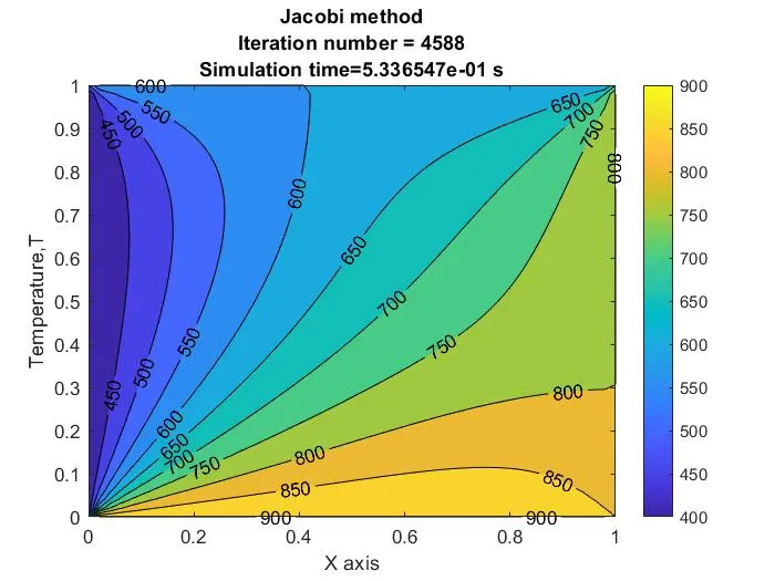
Figure: Jacobi Method
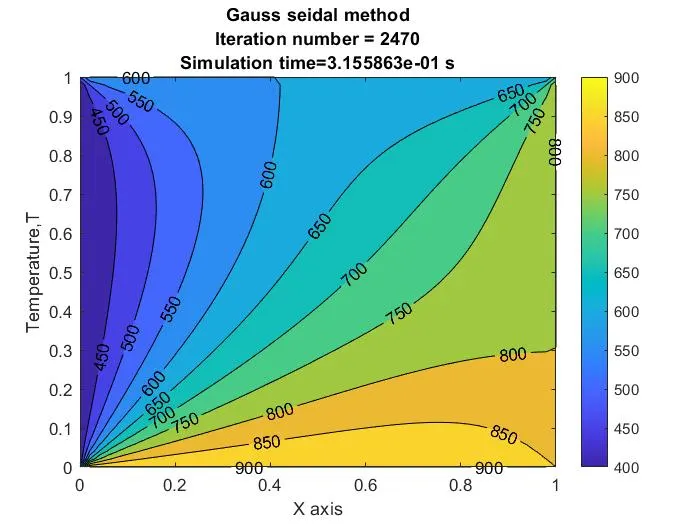
Figure: Gauss-seidel method
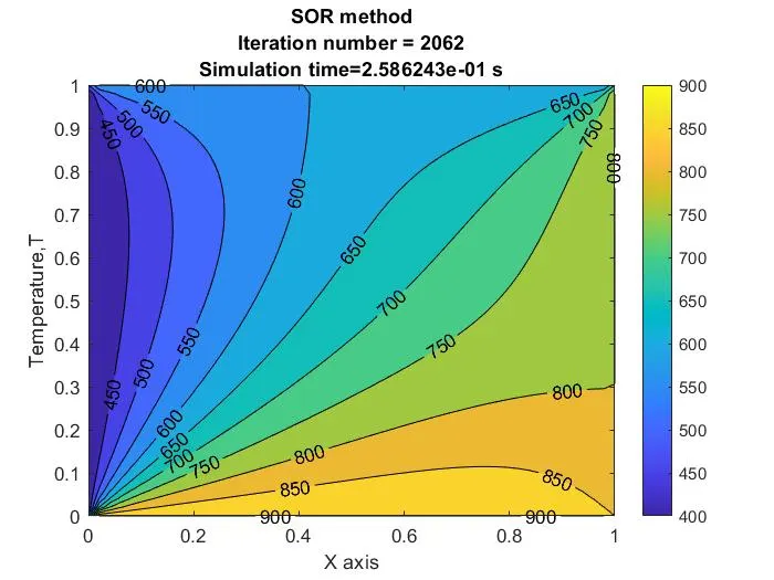
Figure: Successive over-relaxation (SOR) method
From above figures it is found that SOR method has better convergence rate compared to Jacobi method and Gauss-Seidal method.
Again Jacobi method has less congergence rate compared to compared to other two methods.
2) Unsteady state
a) Explicit
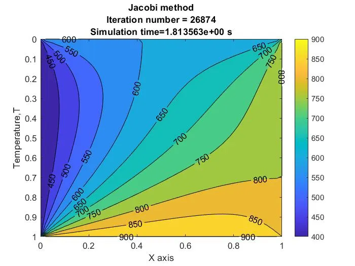
Figure: Jacobi Method
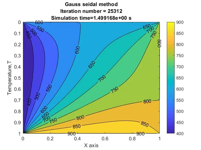
Figure: Gauss-seidel method
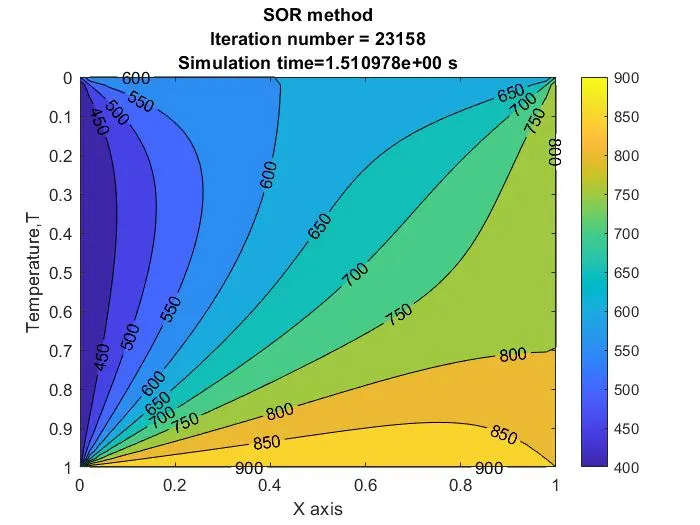
Figure: Successive over-relaxation (SOR) method
In unsteady explicite method also same trend is observed for conevregence rate.
From above figures it is found that SOR method has better convergence rate compared to Jacobi method and Gauss-Seidal method.
Again Jacobi method has less congergence rate compared to compared to other two methods.
b) Implicit
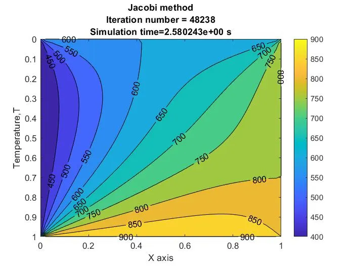
Figure: Jacobi Method
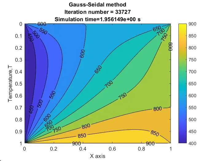
Figure: Gauss-seidel method
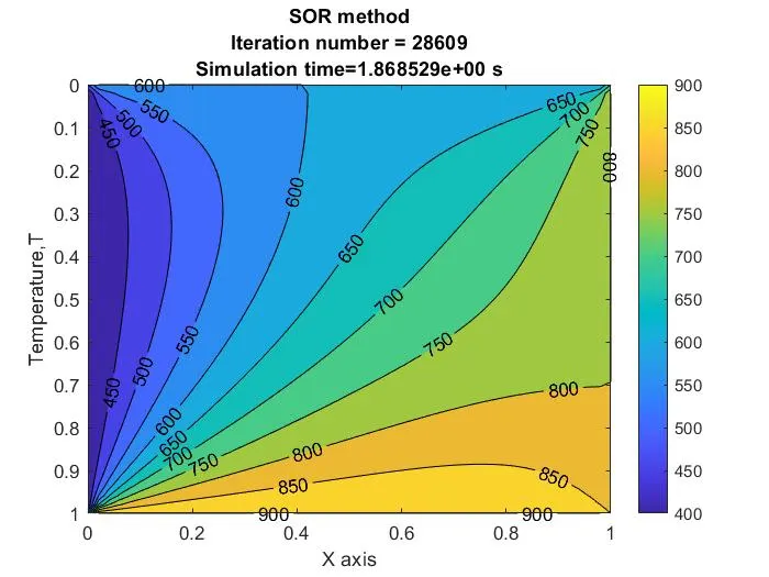
Figure: Successive over-relaxation (SOR) method
As fas as convergence rate is concerned, implicite method has same behaviour as that of explicite nethod.
SOR method has more convergance rate and Jacobi method has least convergance rate and Gauss-Seidal has convergance rate which is between other two methods.
Conclusion
1. Unsteady state simulation takes more time compared steady state simulation for convergance.
2. If we compare explicite and implicte method, explicite method converges faster. But explicite method has linlitation of time step size. If time step size is bigger, solution becomes unstable as bigger time step size increases CFL no. Implicite scheme is unconditinally stable. Even bigger time step size gives stable solution.