Week 3: Flow over a backward facing step

Title: Simulation of flow over backward facing step using Converge CFD.

Aim: To simulate flow over a backward facing step to study velocity and pressure distribution, mass flow rate and floe saperation.

Theory:

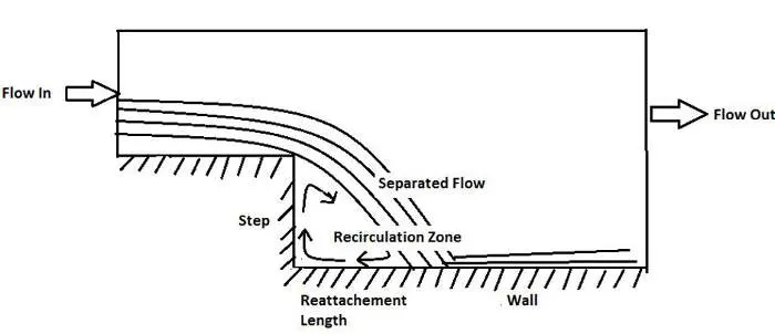
Backward Facing Step (BFS) is widely known for its application in the studies on turbulence in internal flows. The flow separation is caused due to the sudden changes in the geometry. This creates a zone of re-circulation and a point of flow reattachment.

In this problem, Fully developed flow enters the domain from left as shown below. When the flow reaches the step, because of expansion of flow channel, pressure gradient exists, it detaches and a recirculation zone is formed. A turbulent boundary layer encounters a sudden back step, causing flow separation. Later the flow eventually reattaches to the bottom wall.

Importance of Backward Facing Step Problem

Separation and reattachment of turbulent flows occur in many practical engineering applications. It is seen both in internal flow systems such as diffusers, combustors and channels with sudden expansions, and in external flows like flow around airfoil and building. In these situations, the flow experiences an adverse pressure gradient which causes the boundary layer to separate from the solid surface. The flow subsequently reattaches downstream forming a recirculation bubble. The presence of a separated flow, together with a reattaching flow, gives rise to increased unsteadiness, pressure fluctuations which may lead to structure vibrations and noise.

The flow over a backward facing step provides an example of above said flow field. The flow separation and reattachment phenomenon are studied using velocity vector

Geometry:

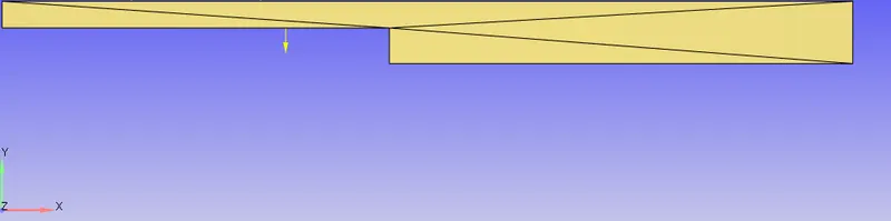
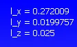
Above geometry is ised for simulation with following diemntions along x, y and z directions respectively.

Set up:

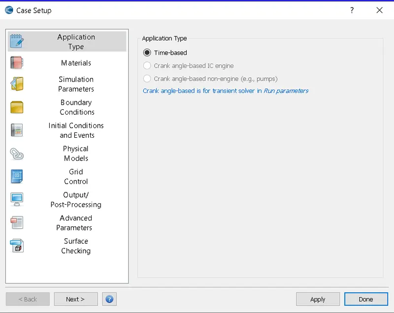
Application type

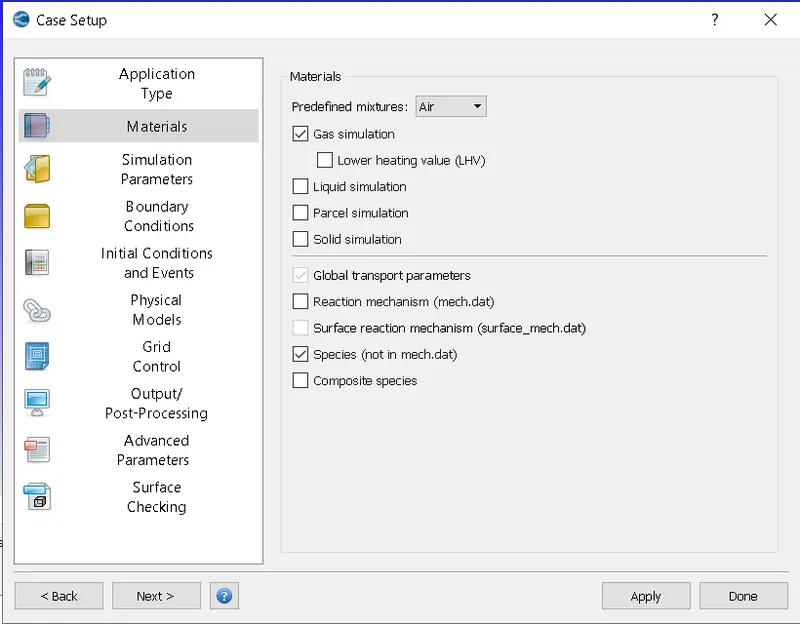
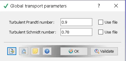
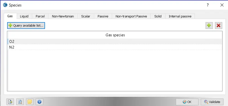
Materials

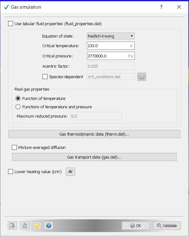
Working fluid is selected as Air

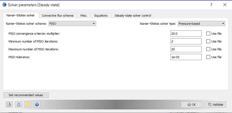
Simulation run parameters

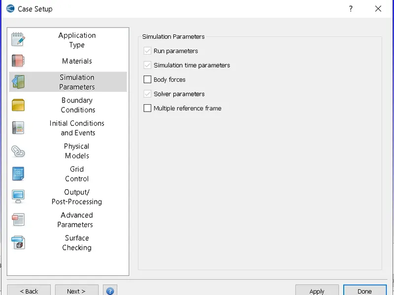
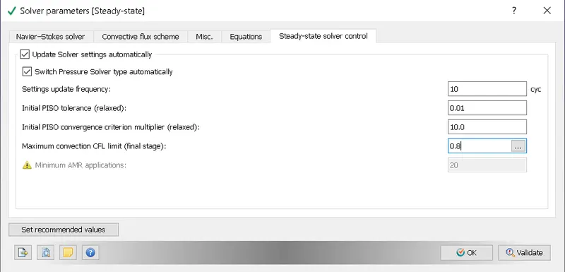
Steady state solver is selecetd with compressible flow simulation

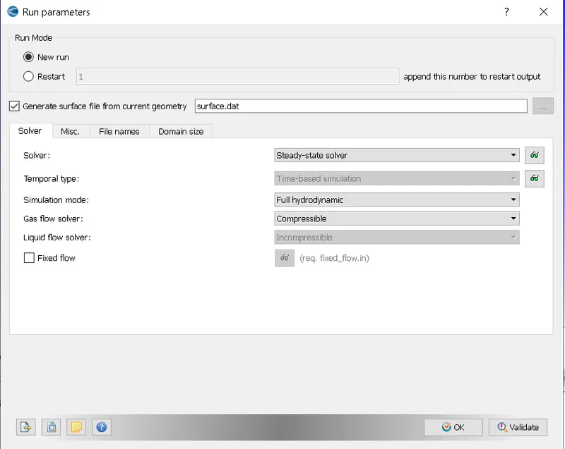
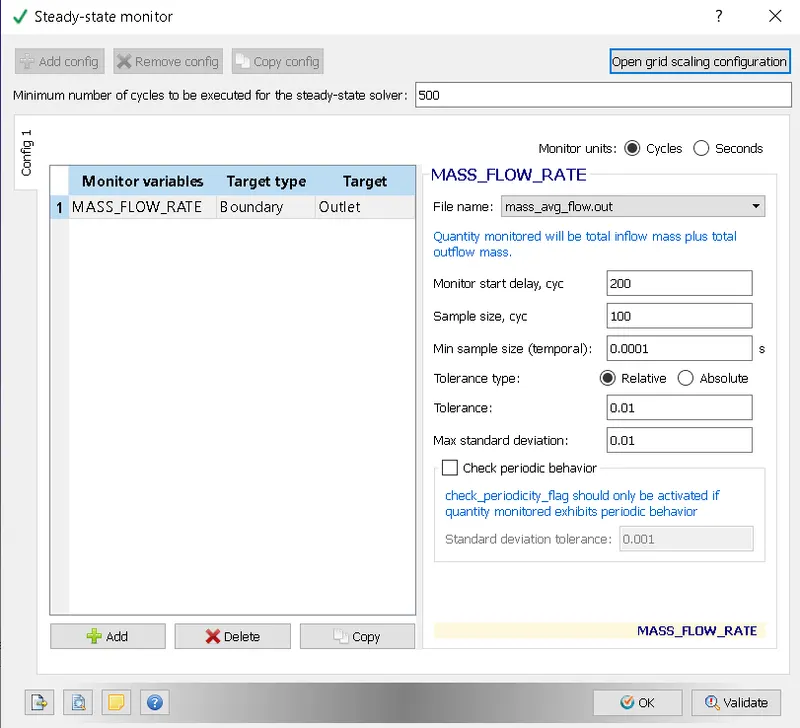
Simulation time = 15000 cyc

Initial time step = 1e-06

Minimum time step = 1e-06

Maximum time step = 2

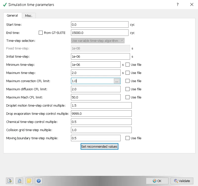
Pressure based solver is selected

Boundary conditions

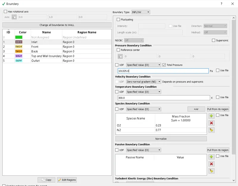
Inlet boundary condition

Pressure: Specified value (101325 Pa)

Velocity boundary: Zero normal gradient

Temperature: Specified value (300 K)

Pressure: Specified value (101325 Pa)

Velocity boundary: Zero normal gradient

Temperature: Specified value (300 K)

Outlet boundary condition

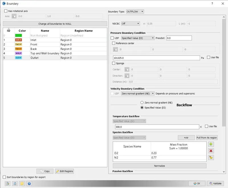
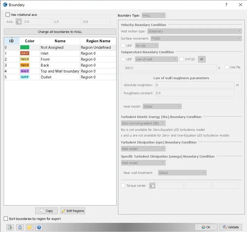
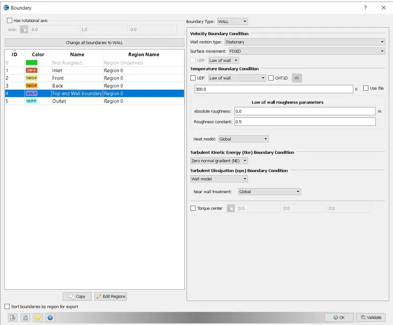
Wall boundary condition

Wall motion type: Stationary

Surface movement: Fixed

Temperature: Specified wall (300 K)

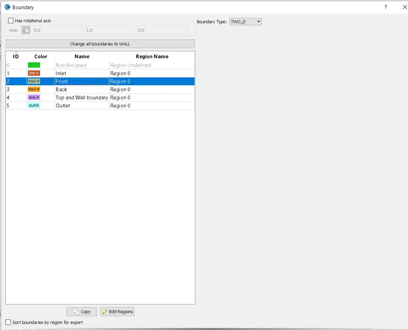
Front and back boundary condition

Dimentions along Z directions are infinite. Hence there are no gradients along Z directions and flow is considered to be 2D (along x and y direction). Hence flow is considered to be 2D by specifying TWO_D boundary.

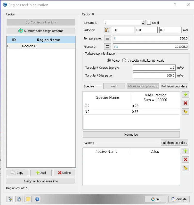
Regions and initialisation

Initial temeperature throughout the domain: 300K

Initial Pressure throughout the domain: 101325 Pa

Physical models

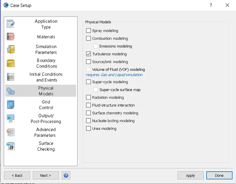
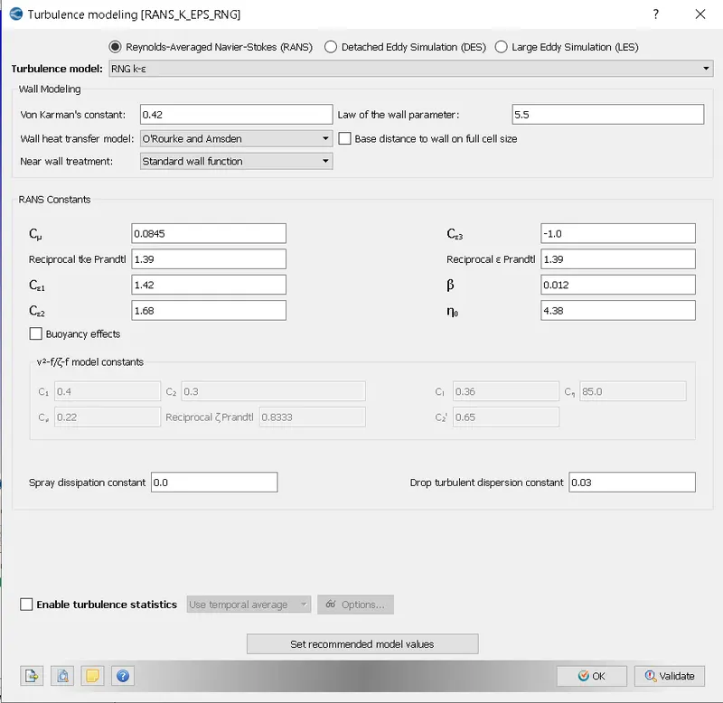
RNG k-e model is considered

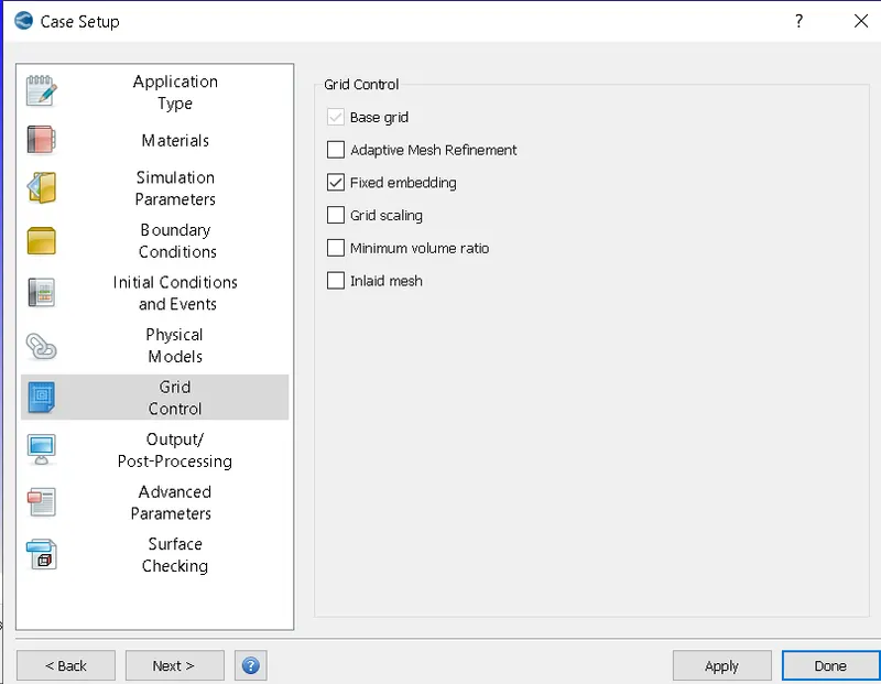
Grid controll

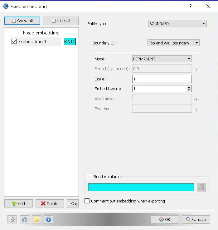
Fixed embeding option is enabled

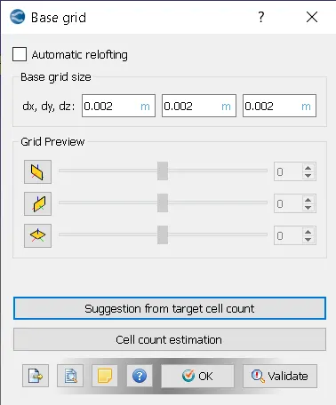
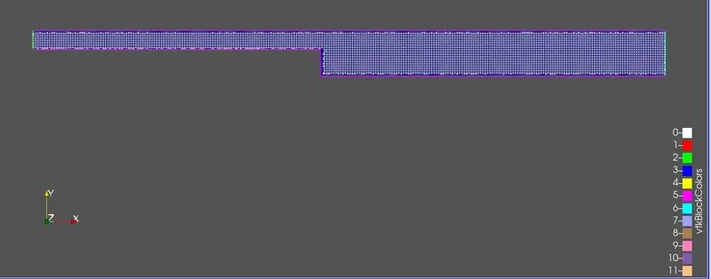
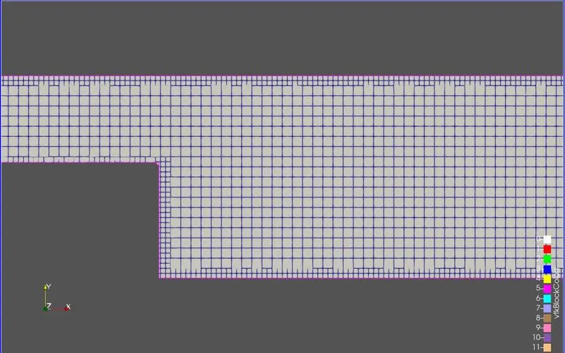
3 kinds of grids are created with mesh size of 2e-3 m, 1.5e-3 m and 1e-3 m as shown in figure.

Results

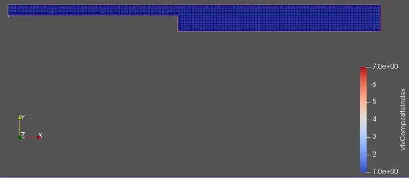
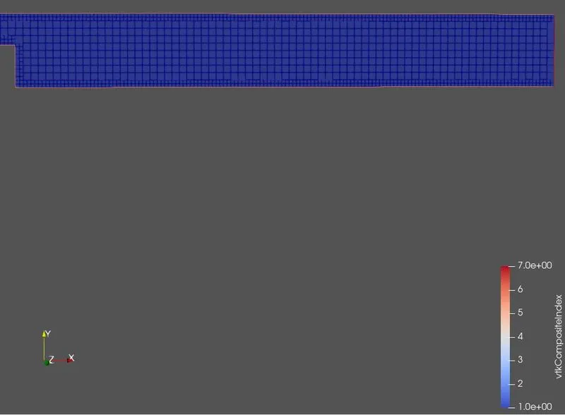
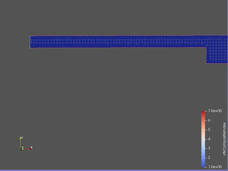
1) Mesh size = 2e-3 m

Mesh

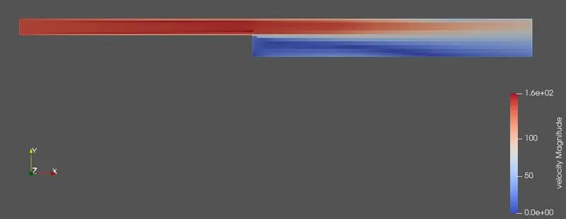
Velocity contours

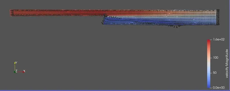
Velocity vectors

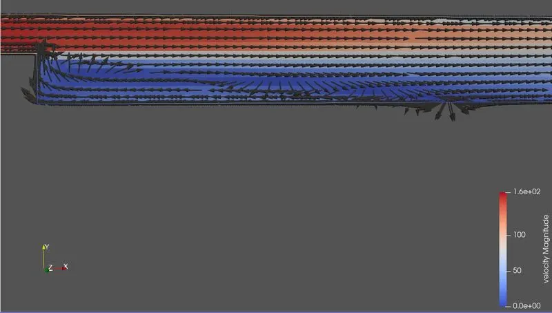
Recirculation region

Velocity animation: https://youtu.be/QTlCx6EbdJk

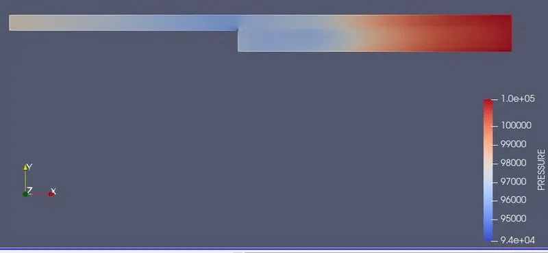
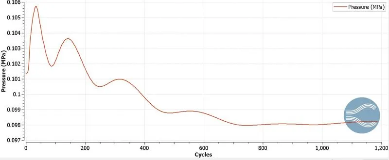
Pressure contour:

Pressure animation: https://youtu.be/HiNFAUpDCxI

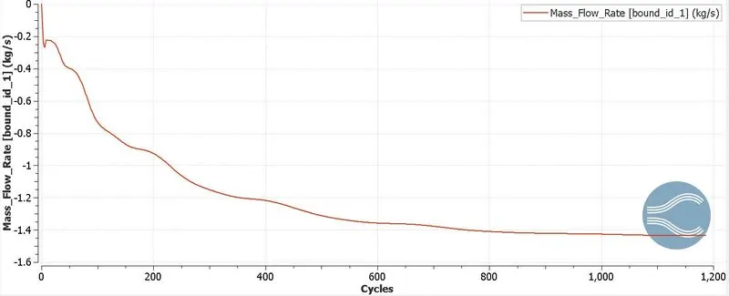
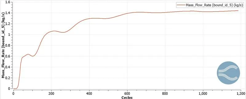
Mass flow rate

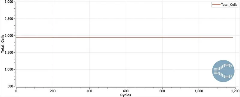
Total cells

2) Mesh size = 1.5e-3 m

Mesh

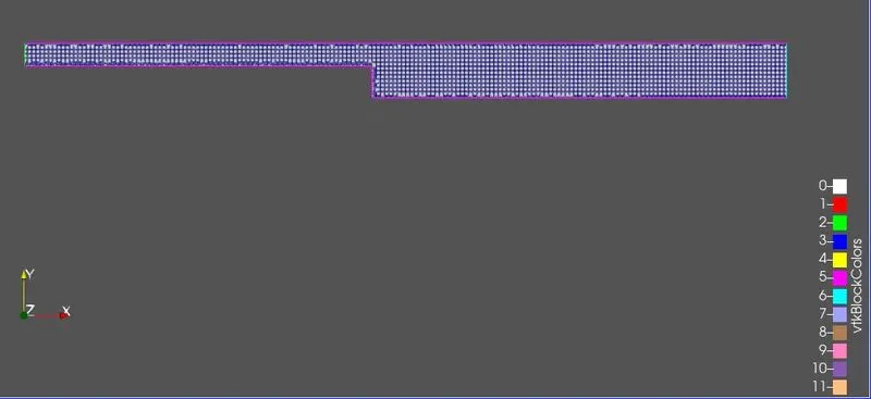
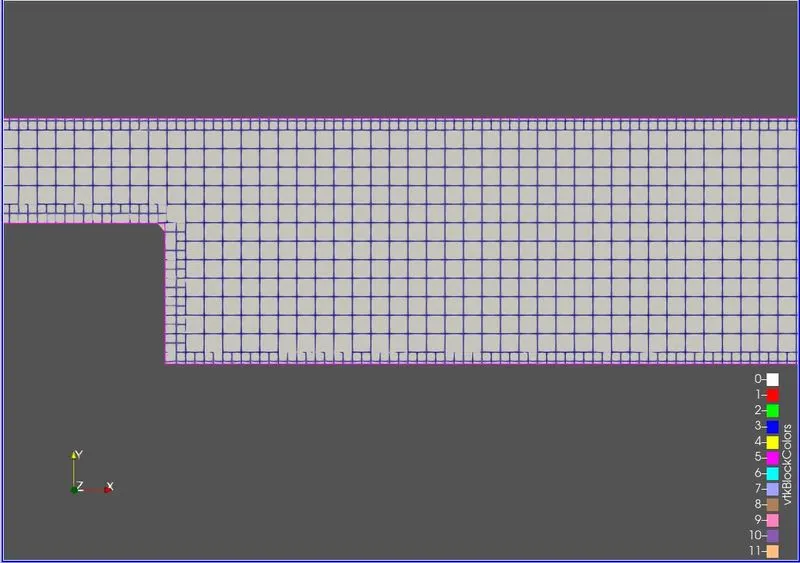
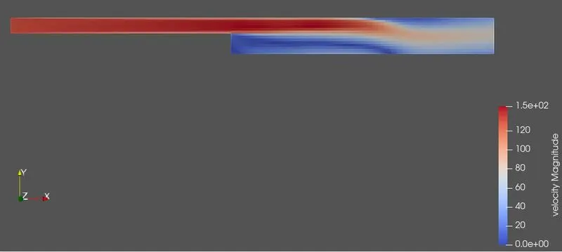
Velocity contours

Velocity vectors

Recirculation region

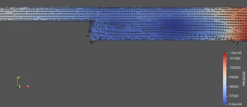
Velocity animation: https://youtu.be/kCjuGJDcolA

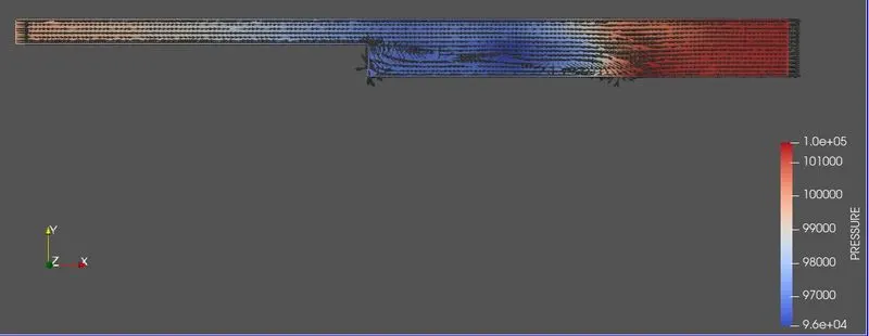
Pressure contour:

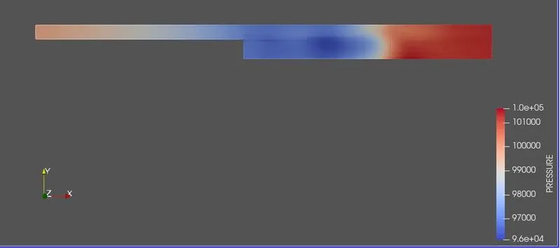
Pressure animation: https://youtu.be/B_vkFMYkTxg

Mass flow rate

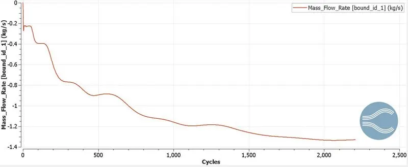
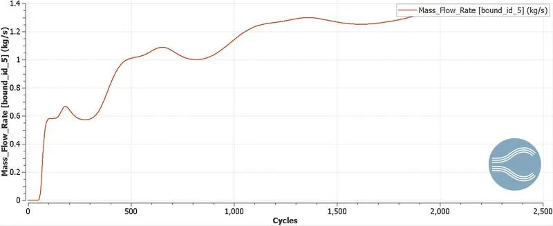
Total cells

3) Mesh size = 1e-3 m

Mesh

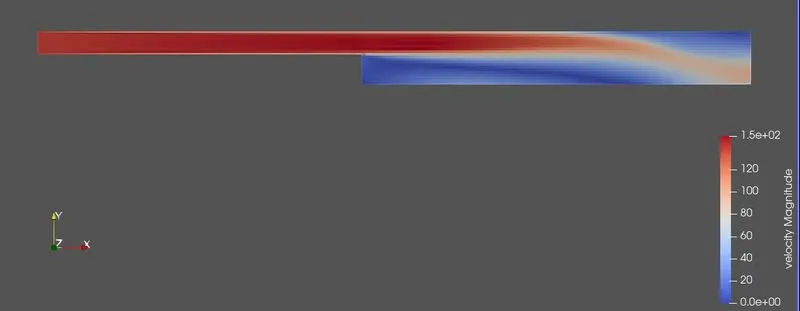
Velocity contour

Velocity vector

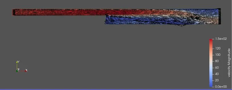
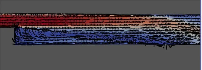
Recirculation region

Velocity animation: https://youtu.be/WdeDZqJATaw

Pressure contour

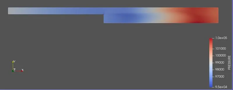
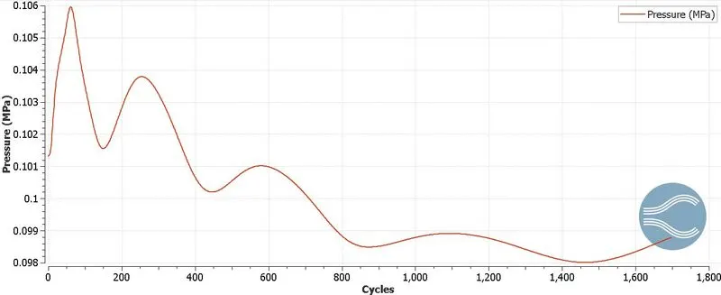
Pressure animation: https://youtu.be/4Civ7q8NbsU

Mass flow rate

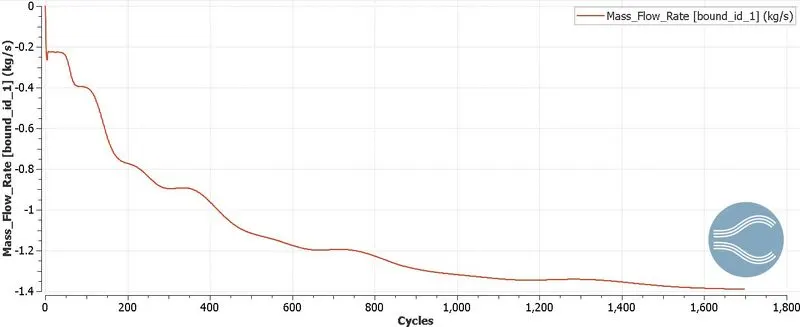
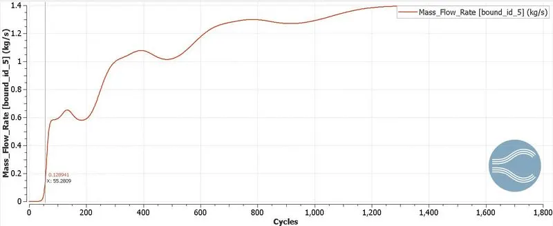
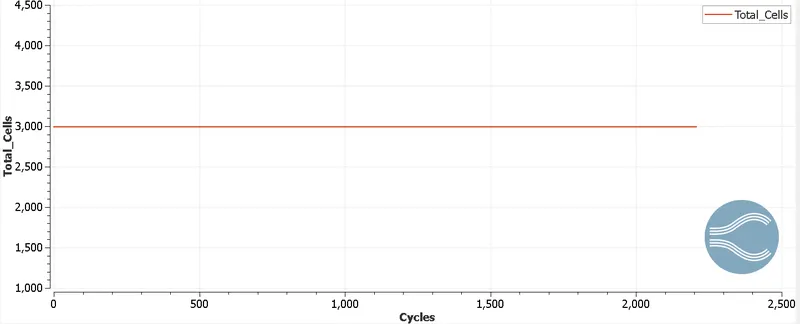
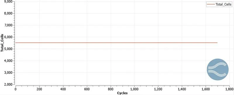
Total cell

Results and discussion

• As mesh size decreses, solution time increses and contours become more and more smooth.
• Velocity is more in the upstream of step becuase of less flow crossectional area.
• After fluid crosses step, there is suddent increased in flow area, as a result there is a flow saperation, and recirculation region forms.
• After step, at a certain distance, flow reattaches again with the wall/surface.
• Pressure contour shows, variation of static pressure. Static pressure is less upstream of step and it is more in the downstream of step because of less and higher flow crossectional area repsectively.
• In recirculation zone pressure is less as compared to its downstream neat the end of the domain.