Project 1 - Parsing NASA thermodynamic data

Aim:

• To write MATLAB CODE to extract data from NASA thermodynamic data file.
• To calculate thermodynamic properties like specific heat, enthalpy and entropy for all species present in the data file, from data given in file and to plot variation of specific heat, enthalpy, and entropy of each species with respect to temperature.
• To calculate molecular weight of each species given in a data file.

Introduction:

File parsing means reading data from given file to facilitate some transformation on the data present in the file. In the current project parsing of NASA thermodynamic data is done using MATLAB code. File is present in .dat format. File contains 53 species. Each species has 14 coefficients by using which specific heat, enthalpy and entropy are calculated. Out of 14 coefficients, first 7 are high-temperature coefficients and next 7 are low-temperature coefficients. Also, molecular weight of each species is calculated.

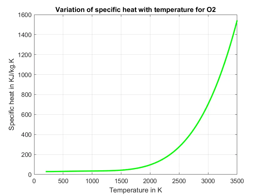
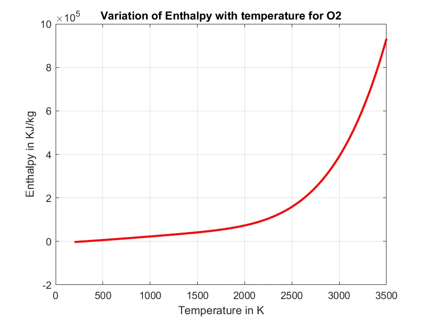
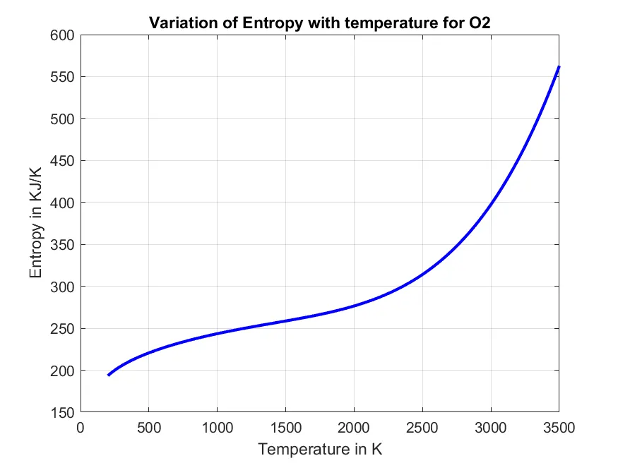
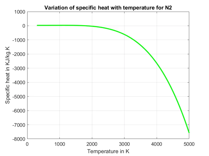
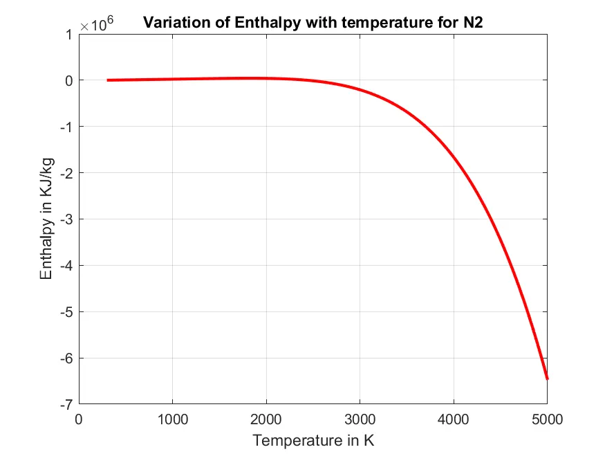
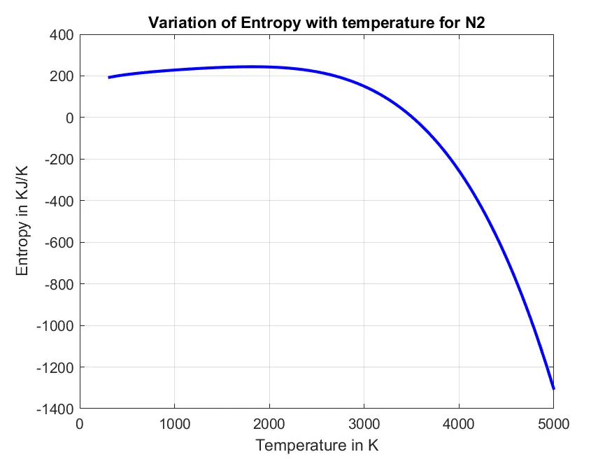
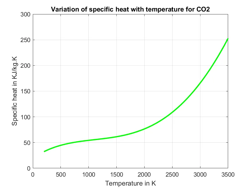
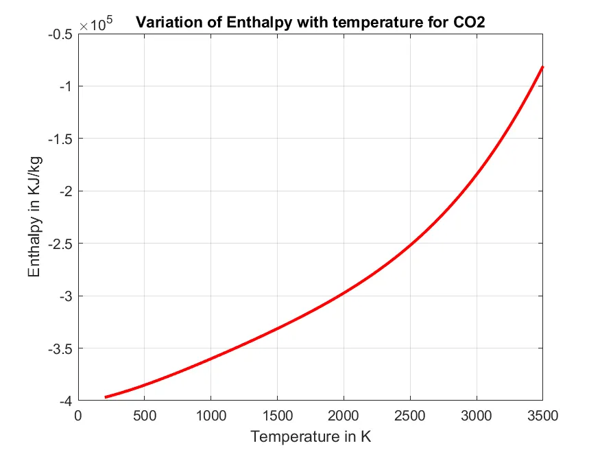
After calculating specific heat, enthalpy and entropy, variation of it is plotted with respect to temperature for each species. Each species will have three plots. So total number of plots are 53x3=159. In the code arrangement is done in a such way that, all plots are saved in single folder species wise separately.

Following mathematical relations are used to calculate specific heat, enthalpy, and entropy, respectively.

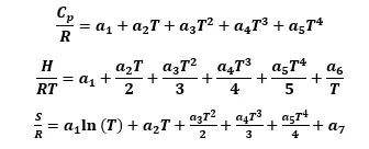
Where Cp is specific heat at constant pressure, R is universal gas constant, H is enthalpy, S is entropy and T is temperature.

Code explanation

1. Given .dat file is read by using ‘fopen(' THERMO.dat', 'r')

   f1 = fopen('THERMO.dat', 'r');​

2. By using ‘fget(l)’ command, first line (THERMO)is read.

   fgetl(f1);​

3. Global temperatures (2^nd line of file) is read by using ‘aa = fgetl(f1)’. Then this line is spitted by using ‘fget(l)’ command. Then global temperatures (300, 1000 and 5000) are read.

   aa = fgetl(f1);
   tt = strsplit(aa, ' ');
   global_low_temp = str2num(tt{2});
   global_mid_temp = str2num(tt{3});
   global_high_temp = str2num(tt{4});
   

4. Line no 3, 4 and 5 are read using ‘fget(l)’ command.

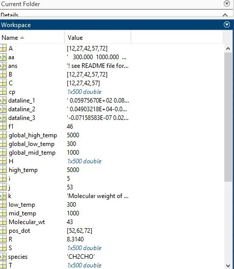
    To eliminate comment lines
   for i=3:5
        fgetl(f1);
   end​

5. Now each species has 4 lines. First line contains the species name and local temperatures (low, middle and high temperature). Next line

   (O L 1/90O 1 G 200.000 3500.000 1000.000 1)

   is read by using ‘fget(l)’ command. Then to identify the species, above line is splitted using ‘fget(l)’ command and name species is identified.

   for j=1:53
   tline=fgetl(f1);
   A = strsplit(tline, ' ');
   species = (A{1});​

6. Now to determine the values of low, middle, and high temperature, the location of dot(.) is identified and with respect to position of dot(.) values of low, middle, and high temperature are read.

   pos_dot=strfind(tline,'.');
   low_temp = tline(pos_dot(1)-3:pos_dot(1)+3);
   low_temp = str2num(low_temp);
   high_temp = tline(pos_dot(2)-4:pos_dot(2)+3);
   high_temp =  str2num(high_temp);
   mid_temp = tline(pos_dot(3)-4:pos_dot(3)+3);
   mid_temp =  str2num(mid_temp);​

7. Similarly, next 3 lines are read using ‘fget(l)’ command. First and second line has 5 coefficients each and 3^rd line has 4 coefficients. To read value of each coefficient, position of ‘E’ has been found out in each line and with respect to position of ‘E’ each coefficient value is read.

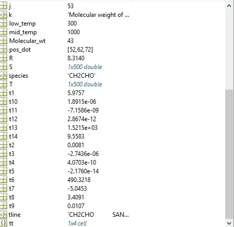
   dataline_1 = fgetl(f1);
   dataline_2 = fgetl(f1);
   dataline_3 = fgetl(f1);
   
   A = strfind(dataline_1,'E');
   B = strfind(dataline_2,'E');
   C = strfind(dataline_3,'E');​

8. Then function code is written to calculate specific heat, enthalpy, entropy and molecular weight.

   function cp = specific_heat(t1,t2,t3,t4,t5,t6,t7,t8,t9,t10,t11,t12,t13,t14,T,R,low_temp,high_temp,mid_temp)
   if T>mid_temp
       cp = (t1+t2.*(T)+t3.*(T.^2)+t4.*(T.^3)+t5.*(T.^4))*R;
   else
       cp = (t8+t9.*(T)+t10.*(T.^2)+t11.*(T.^3)+t12.*(T.^4))*R;
   end
   end​

   function [H] = enthalpy(t1,t2,t3,t4,t5,t6,t7,t8,t9,t10,t11,t12,t13,t14,T,R,low_temp,high_temp,mid_temp)
   if T>mid_temp
       H = (t1.*T+t2.*(T.^2)./2+t3.*(T.^3)./3+t4.*(T.^4)./4+t5.*(T.^5)./5+t6)*R;
   else
       H = (t8.*T+t9.*(T.^2)./2+t10.*(T.^3)./3+t11.*(T.^4)./4+t12.*(T.^5)./5+t13)*R;
   end
   end

   function S = entropy(t1,t2,t3,t4,t5,t6,t7,t8,t9,t10,t11,t12,t13,t14,T,R,low_temp,high_temp,mid_temp)
   if T>mid_temp
       S = (t1.*log(T)+t2.*T+t3.*(T.^2)./2+t4.*(T.^3)./3+t5.*(T.^4)./4+t7)*R;
   else
       S = (t8.*log(T)+t9.*T+t10.*(T.^2)./2+t11.*(T.^3)./3+t12.*(T.^4)./4+t14)*R;
   end
   end

   function[molecular_weight] = molecular_weight(species)
   elements = {'H','C','O','N','A','S'};
   atomic_weight = [1,12,16,14,39,32];
   molecular_weight=0;
    for i=1:length(species)
        for j=1:length(elements)
            if strcmp(species(i),elements(j))
                molecular_weight = molecular_weight+atomic_weight(j) 
                a=j;
            end
            end  
          n = str2num(species(i));
          if(n>1)
                molecular_weight = molecular_weight+(atomic_weight(a)*(n-1))
        end
    end
   end

9. Temperature values are specified using ‘linspace’ command and value of R is defined.

   T = linspace(low_temp, high_temp,500);
   R = 8.314;​

10. Specific heat, enthalpy and entropy are calculated.

    % specific heat calculation
    cp = specific_heat(t1,t2,t3,t4,t5,t6,t7,t8,t9,t10,t11,t12,t13,t14,T,R,low_temp,high_temp,mid_temp);
    
    % Entahlpy calculation
    H = enthalpy(t1,t2,t3,t4,t5,t6,t7,t8,t9,t10,t11,t12,t13,t14,T,R,low_temp,high_temp,mid_temp);
    
    % Entropy calculation
    S = entropy(t1,t2,t3,t4,t5,t6,t7,t8,t9,t10,t11,t12,t13,t14,T,R,low_temp,high_temp,mid_temp);

11. Then variation of specific heat, enthalpy and entropy are plotted with respect to temperature.

    % To plot varation of cp with T
    figure(1)
    plot(T, cp, 'linewidth',2,'color','g')
    xlabel('Temperature in K')
    ylabel('Specific heat in KJ/kg.K')
    grid on
    title(sprintf('Variation of specific heat with temperature for %s', species))
    saveas(figure(1),'cp.png');
    
    % To plot variation of enthapy with temperarure
    figure(2)
    plot(T, H, 'linewidth',2,'color','r')
    xlabel('Temperature in K')
    ylabel('Enthalpy in KJ/kg')
    grid on
    title(sprintf('Variation of Enthalpy with temperature for %s', species))
    saveas(figure(2),'H.png');
    
    % To plot variation of entropy with temperarure
    figure(3)
    plot(T, S, 'linewidth',2,'color','b')
    xlabel('Temperature in K')
    ylabel('Entropy in KJ/K')
    grid on
    title(sprintf('Variation of Entropy with temperature for %s', species))
    saveas(figure(3),'S.png');​

12. Molecular weight is calculated.

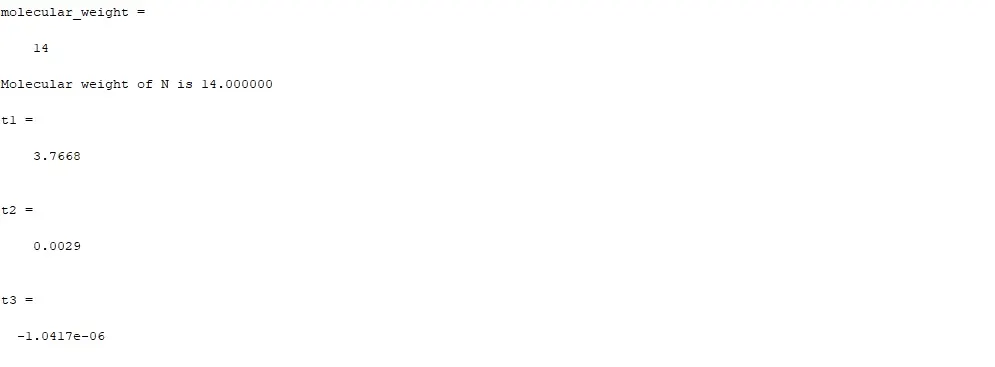
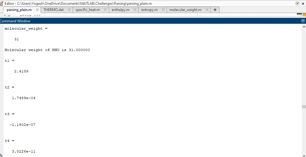
    % To calculate molecular weight
     Molecular_wt = molecular_weight(species);
     k = sprintf('Molecular weight of %s is %f', species,Molecular_wt);
     disp(k)​

13. One folder is created named ‘species’ and all plots are saved in that folder, species wise separately.

    % Saving in a folder
    cd('C:\Users\Yogesh\OneDrive\Documents\MATLAB\species')
    mkdir(species);
    cd(species);​

Complete code:

clear all
close all
clc

% Getting data from provided file
f1 = fopen('THERMO.dat', 'r');
fgetl(f1);
aa = fgetl(f1);
tt = strsplit(aa, ' ');
global_low_temp = str2num(tt{2});
global_mid_temp = str2num(tt{3});
global_high_temp = str2num(tt{4});

% To eliminate comment lines
for i=3:5
     fgetl(f1)
end

% To get species data 
for j=1:53
    tline=fgetl(f1);
    A = strsplit(tline, ' ');
    species = (A{1});
    pos_dot=strfind(tline,'.');
    low_temp = tline(pos_dot(1)-3:pos_dot(1)+3);
    low_temp = str2num(low_temp);
    high_temp = tline(pos_dot(2)-4:pos_dot(2)+3);
    high_temp =  str2num(high_temp);
    mid_temp = tline(pos_dot(3)-4:pos_dot(3)+3);
    mid_temp =  str2num(mid_temp);
    
    dataline_1 = fgetl(f1);
    dataline_2 = fgetl(f1);
    dataline_3 = fgetl(f1);

    A = strfind(dataline_1,'E');
    B = strfind(dataline_2,'E');
    C = strfind(dataline_3,'E');

    t1 = dataline_1(1:A(1)+3);
    t1 = str2num(t1)
    t2 = dataline_1(A(1)+4:A(2)+3);
    t2 = str2num(t2)
    t3 = dataline_1(A(2)+4:A(3)+3);
    t3 = str2num(t3)
    t4 = dataline_1(A(3)+4:A(4)+3);
    t4 = str2num(t4)
    t5 = dataline_1(A(4)+4:A(5)+3);
    t5 = str2num(t5)

    t6 = dataline_2(1:B(1)+3);
    t6 = str2num(t6)
    t7 = dataline_2(B(1)+4:B(2)+3);
    t7 = str2num(t7)
    t8 = dataline_2(B(2)+4:B(3)+3);
    t8 = str2num(t8)
    t9 = dataline_2(B(3)+4:B(4)+3);
    t9 = str2num(t9)
   t10 = dataline_2(B(4)+4:B(5)+3);
   t10 = str2num(t10)

   t11 = dataline_3(1:C(1)+3);
   t11 = str2num(t11)
   t12 = dataline_3(C(1)+4:C(2)+3);
   t12 = str2num(t12)
   t13 = dataline_3(C(2)+4:C(3)+3);
   t13 = str2num(t13)
   t14 = dataline_3(C(3)+4:C(4)+3);
   t14 = str2num(t14)


T = linspace(low_temp, high_temp,500);
R = 8.314;

% specific heat calculation
cp = specific_heat(t1,t2,t3,t4,t5,t6,t7,t8,t9,t10,t11,t12,t13,t14,T,R,low_temp,high_temp,mid_temp);

% Entahlpy calculation
H = enthalpy(t1,t2,t3,t4,t5,t6,t7,t8,t9,t10,t11,t12,t13,t14,T,R,low_temp,high_temp,mid_temp);

% Entropy calculation
S = entropy(t1,t2,t3,t4,t5,t6,t7,t8,t9,t10,t11,t12,t13,t14,T,R,low_temp,high_temp,mid_temp);

% Saving in a folder
cd('C:\Users\Yogesh\OneDrive\Documents\MATLAB\species')
mkdir(species);
cd(species);

% To plot varation of cp with T
figure(1)
plot(T, cp, 'linewidth',2,'color','g')
xlabel('Temperature in K')
ylabel('Specific heat in KJ/kg.K')
grid on
title(sprintf('Variation of specific heat with temperature for %s', species))
saveas(figure(1),'cp.png');

% To plot variation of enthapy with temperarure
figure(2)
plot(T, H, 'linewidth',2,'color','r')
xlabel('Temperature in K')
ylabel('Enthalpy in KJ/kg')
grid on
title(sprintf('Variation of Enthalpy with temperature for %s', species))
saveas(figure(2),'H.png');

% To plot variation of entropy with temperarure
figure(3)
plot(T, S, 'linewidth',2,'color','b')
xlabel('Temperature in K')
ylabel('Entropy in KJ/K')
grid on
title(sprintf('Variation of Entropy with temperature for %s', species))
saveas(figure(3),'S.png');
 
cd('C:\Users\Yogesh\OneDrive\Documents\MATLAB\species')
 
% To calculate molecular weight
 Molecular_wt = molecular_weight(species);
 k = sprintf('Molecular weight of %s is %f', species,Molecular_wt);
 disp(k)
    
end

All plots are saved in a folder named 'species' saperately

Images present in a folder

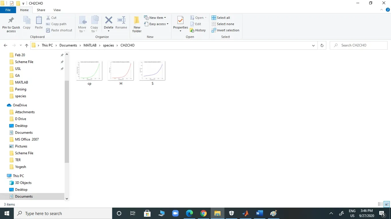
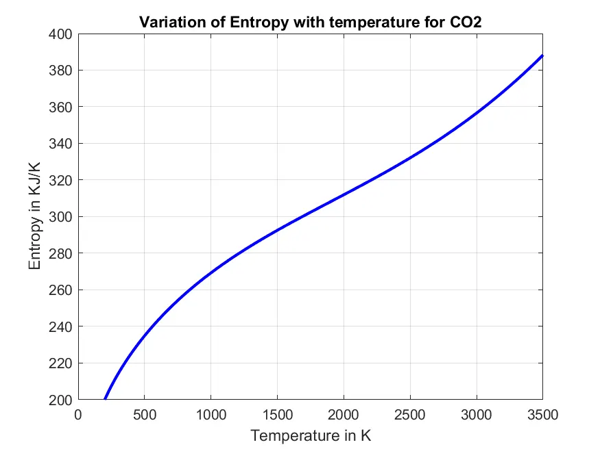
Varaition of speciffic heat, enthalpy and entropy for O2, N2 and CO2.

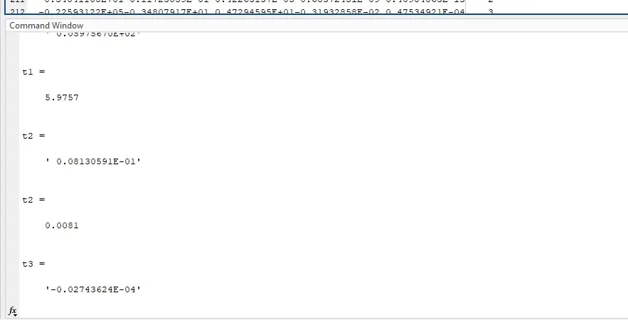
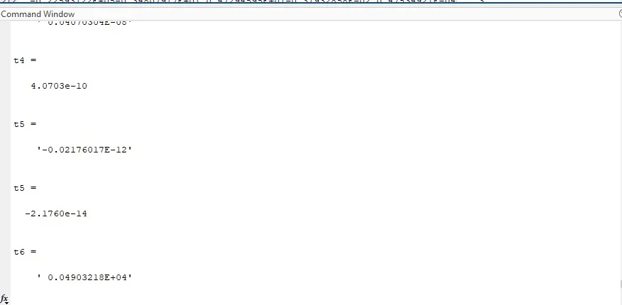
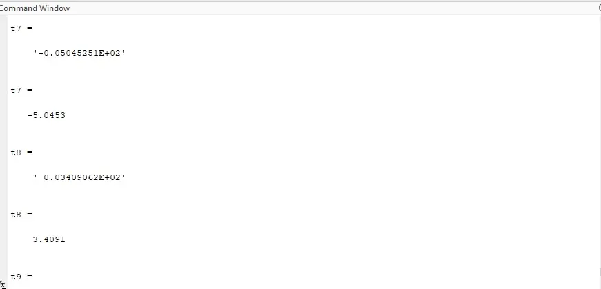
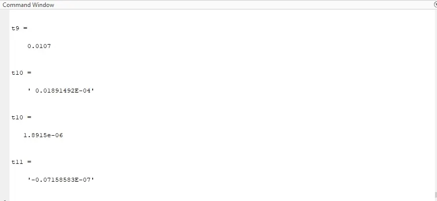
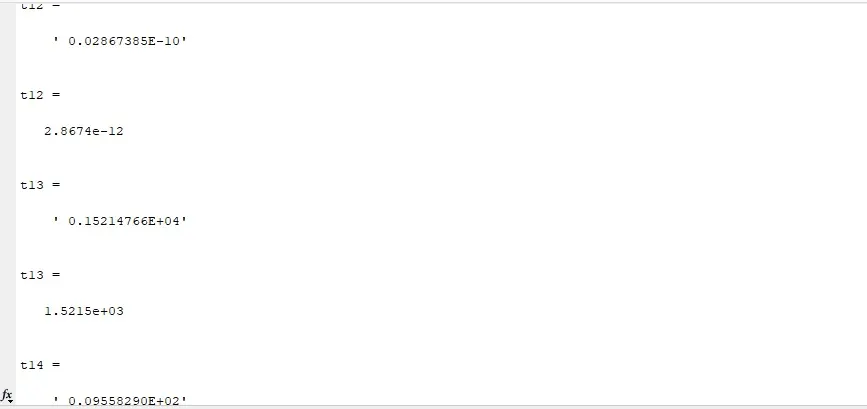
Values of coeficient for CH2CHO

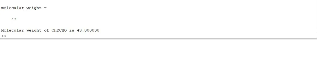
Molecular weight results:

Results: