Week 5: Prandtl Meyer Shock problem
Title: Simulation of Prandtl Meyer Shock problem using converge CFD.
Aim: To study the effect of Sub-grid scale (SGS) on shock location and cell count.
Introduction:
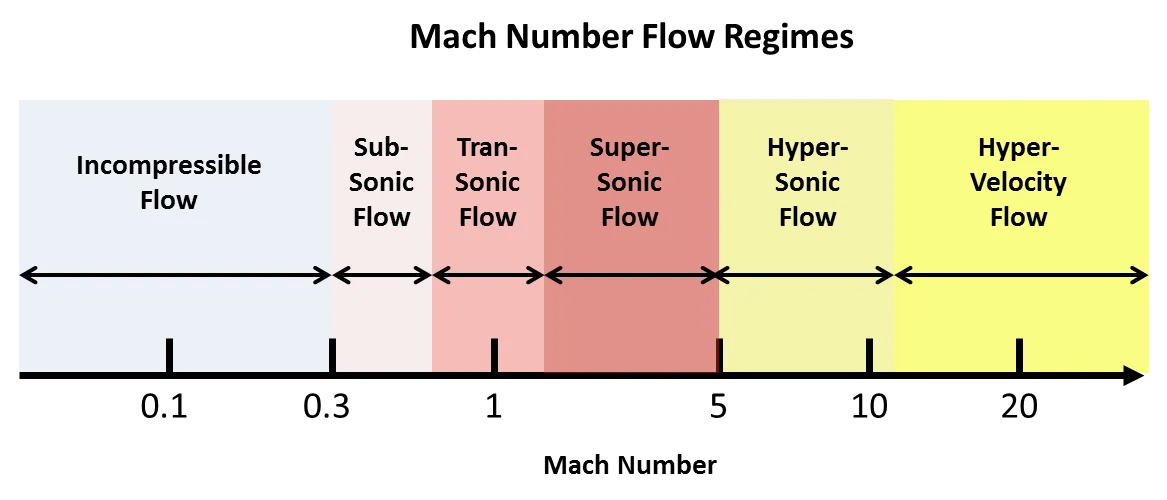
Compressible flow is the branch of Fluid Mechanics that deals with flows having significant changes in fluid density. Flows are treated as compressible when Mach number is more than 0.3. (Mach nunber is a ratio of speed of the flow to the speed of sound), since in this case density chamges are less than 5% due to velocity. The study of compressible flow is relevant to high-speed aircraft, jet engines, rocket motors, high-speed entry into a planetary atmosphere, gas pipelines, commercial applications such as abrasive blasting, and many other fields.
Depending upon the magnitude of Mach number, flow may be incompressible or compressible (subsonic, transonic, supersonic, hypersonic or hypervelocity flow) as shown below.
Introduction to shock wave
Shock wave or shock, is a type of propagating disturbance that moves faster than the local speed of sound in the medium. Like an ordinary wave, a shock wave carries energy and can propagate through a medium. It is characterized by an abrupt, nearly discontinuous, change in pressure, temperature anddensity of the medium. Dependiong upon the relative speed of sourse or object and speed of sound, the nature of propogation of sound changes as shown below.
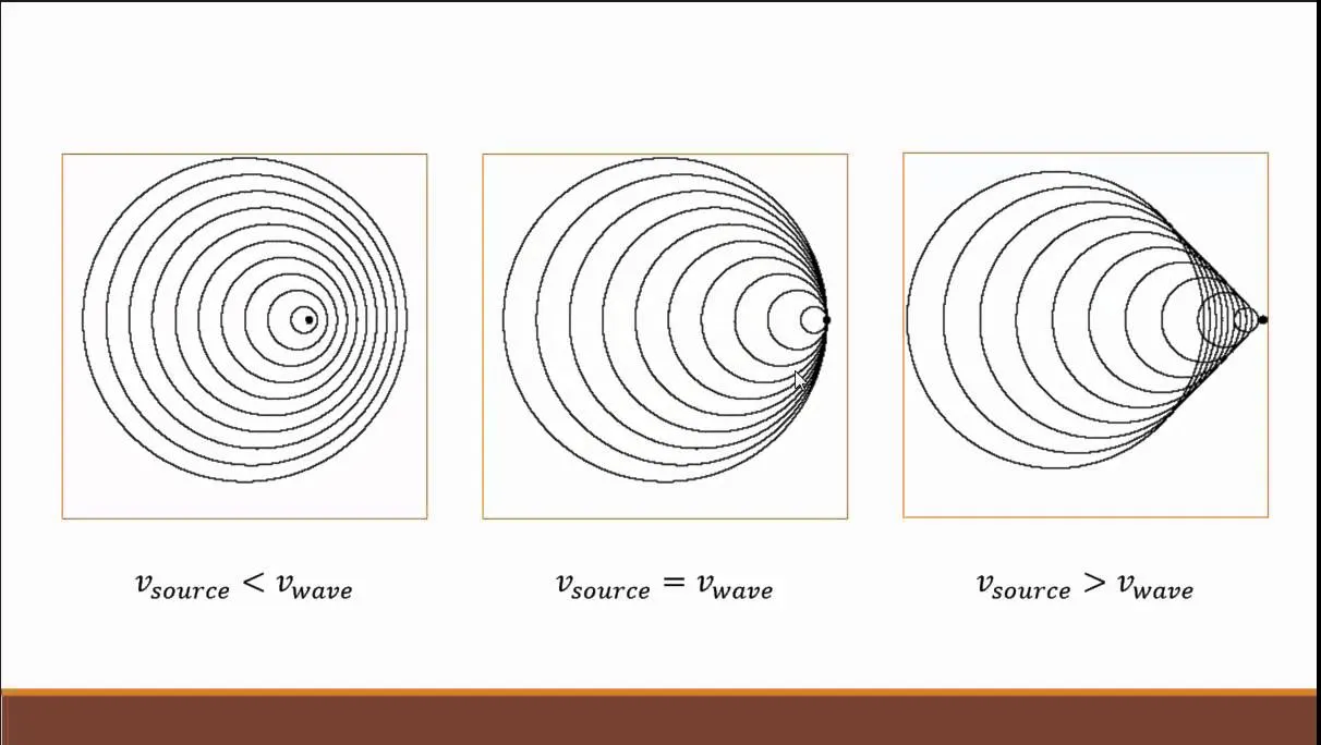
As an object accelerates from subsonic toward supersonic speed in a gas, different types of wave phenomena occur. Stationary point (M = 0) that emits symmetric sound waves. The speed of sound is the same in all directions in a uniform fluid, so these waves are simply concentric spheres. As the sound-generating point begins to accelerate, the sound waves "bunch up" in the direction of motion and "stretch out" in the opposite direction. When the point reaches sonic speed (M = 1), it travels at the same speed as the sound waves it creates. Therefore, an infinite number of these sound waves "pile up" ahead of the point, forming a shock wave. Upon achieving supersonic flow, the particle is moving so fast that it continuously leaves its sound waves behind. When this occurs, the locus of these waves trailing behind the point creates an angle known as the Mach wave angle or Mach angle, μ.
Types of shock waves:
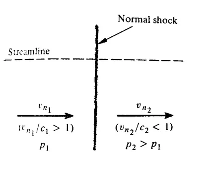
1) Normal shock
A normal shock occurs in front of a supersonic object if the flow is turned by a large amount and the shock cannot remain attached to the body. The detached shock occurs for both wedges and cones. A normal shock is also present in most supersonic inlets.
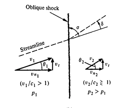
2) Oblique shock
An oblique shock wave is a shock wave that is inclined with respect to the incident upstream flow direction.
Introduction to Prandtl Meyer Shock problem
It is a problem which depicts that, when supersonic flow turns around a convex corner, infinite mach waves are forms and form waves are expanding from a vertex point as shown in figure below.
M = Mach number, `μ = Mach angle`
In this problem, similar kind of geometry is taken and formation of mach wave is studied for different inlet speeds. Also effect of sub-grid scale is studied on the mesh.
Adaptive mesh refinement
In numerical simulations, adaptive mesh refinement (AMR) is a method of adapting the accuracy of a solution within certain sensitive or turbulent regions of simulation, dynamically and during the time the solution is being calculated. In certain regions where more accuracy of solution is needed, it is better if mesh refines automatically in that region keeping mesh in others regions unchanged. This can be achived by adaptive mesh refinement (AMR) technique.
Shock flow boundary conditions:
1. Dirichlet boundary condition
In this type boundary condition, value of variable is specified at boundary. e.g. y = f
2. Neumann boundary condition
In this type boundary condition, gradient of variable is specified at boundary. e.g. `dy/dx=f`
3. Robin boundary condition
It is combination of above 2 boundary conditions.
4. Mixed boundary condition
There is a Dirichlet boundary condition on one boundary and Neumann boundary condition on other body.
At super-sonic outlets neumann boundary condition is used because at outlet values of variables like temperature, pressure, velocity etc are not known before solution of problem. Hence the values of variables are extrapolated from values of variable at interior. However, if values of variable is mentioned at outlet, solution will not converge and will become unstable.
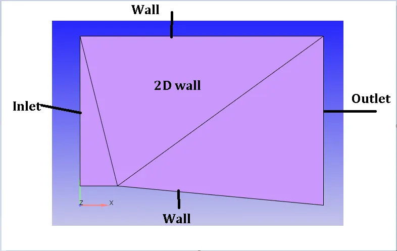
Geometry used in Simulation
Case set-up
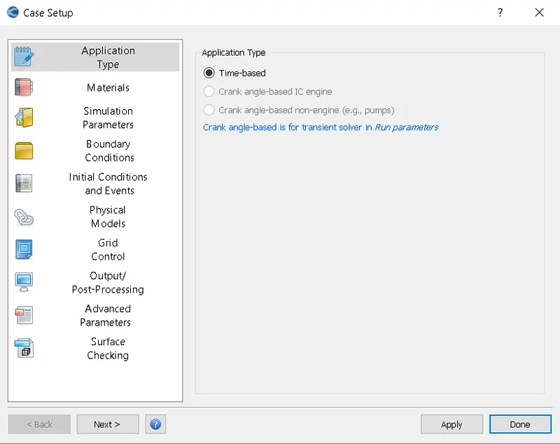
1) Application type
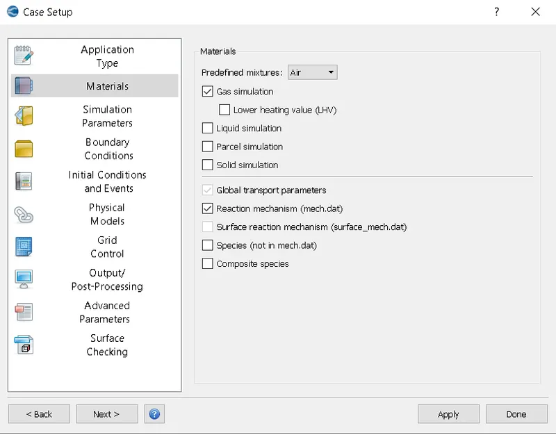
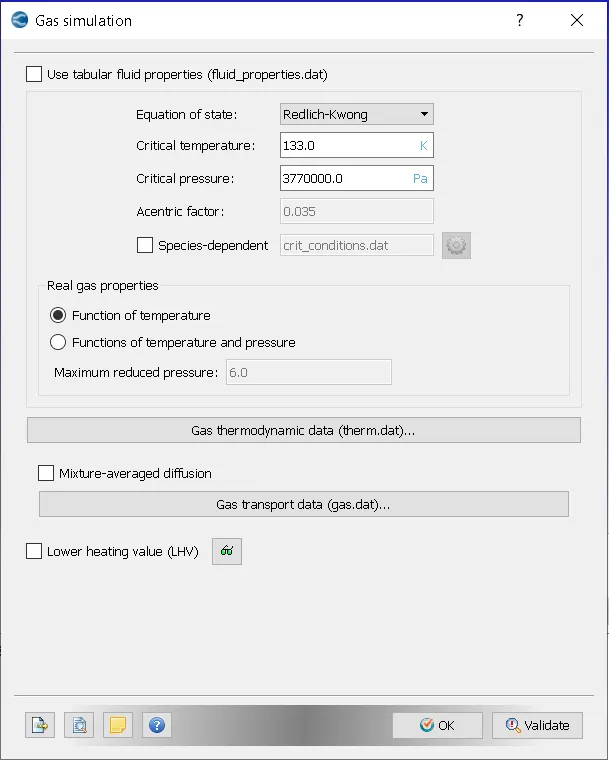
2) Material
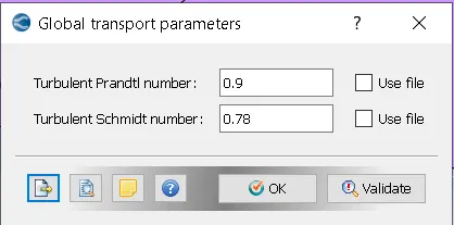
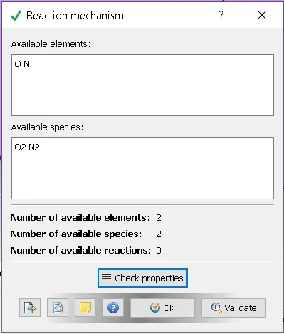
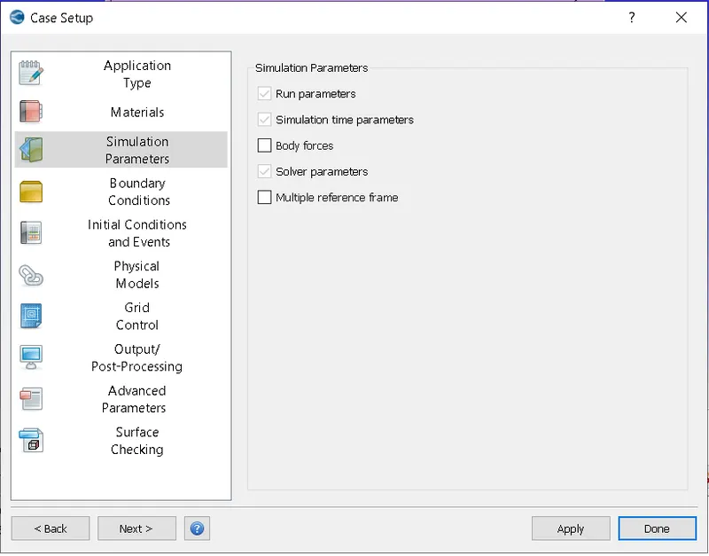
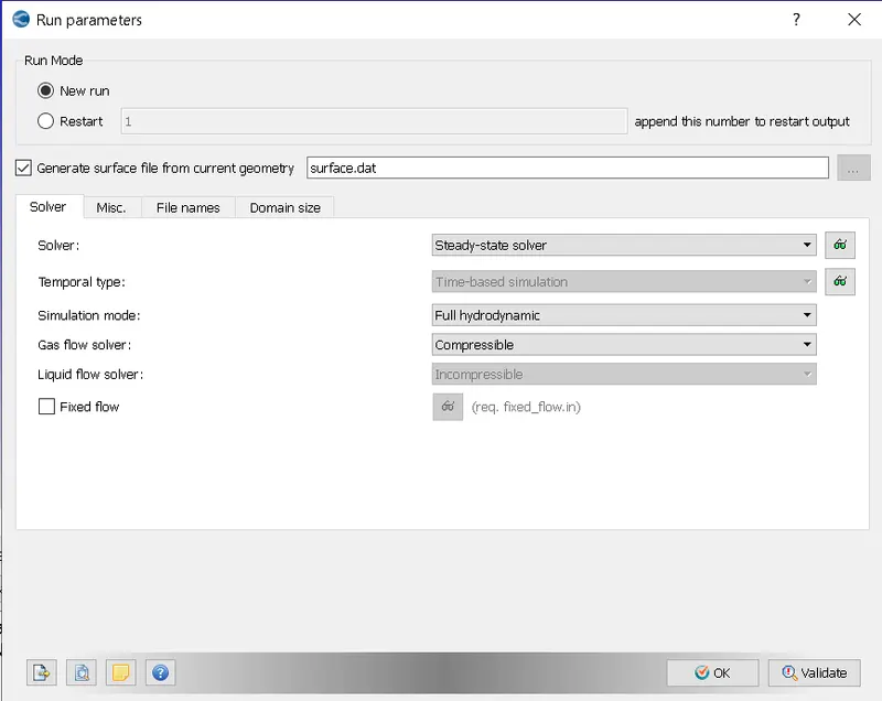
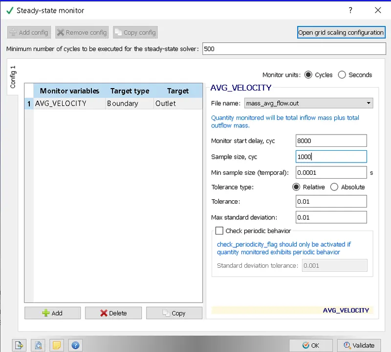
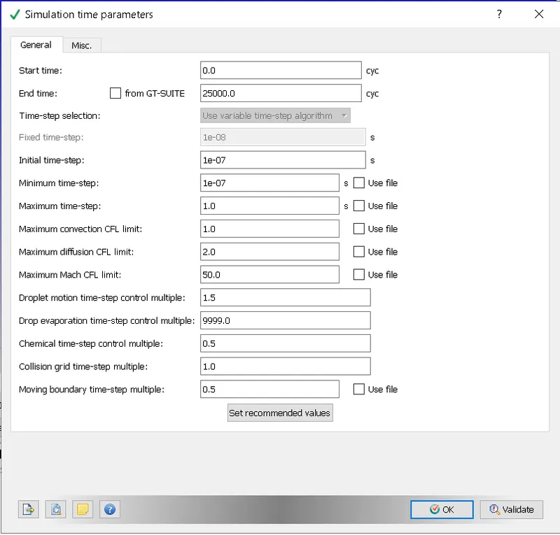
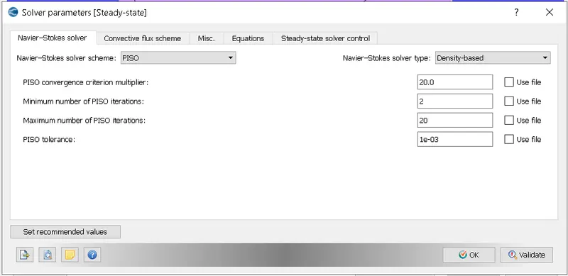
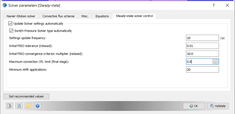
3) Simulation parameters
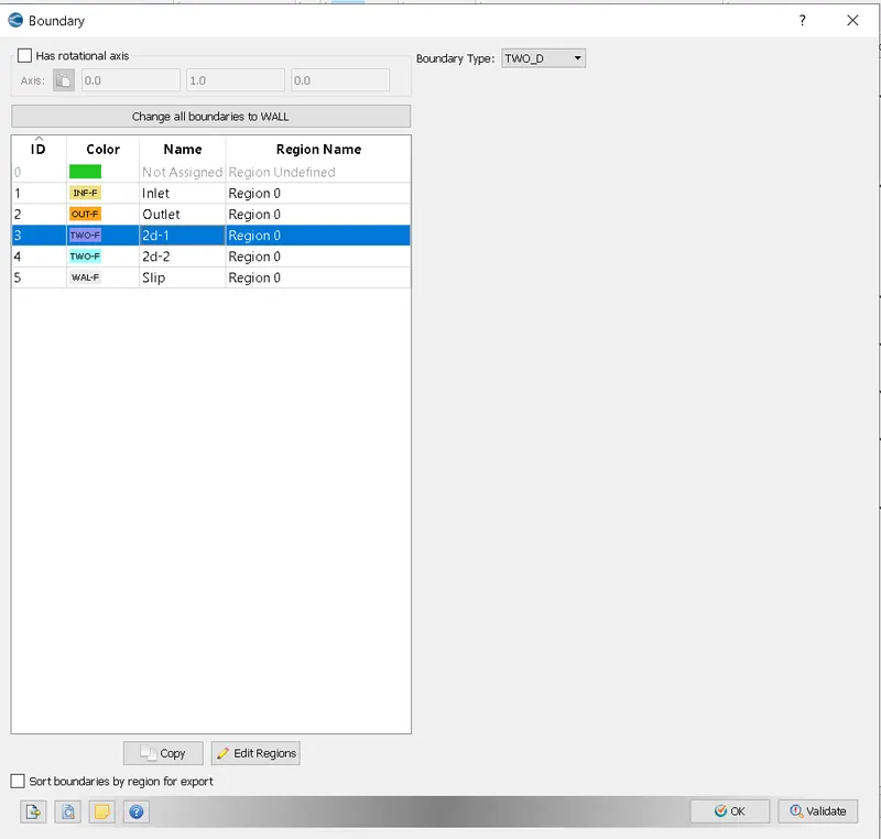
4) Boundary conditions
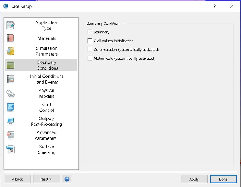
Inlet
Pressure: 101325 Pa
Velocity: 680 m/s or 100 m/s
Temperature: 286.1 K
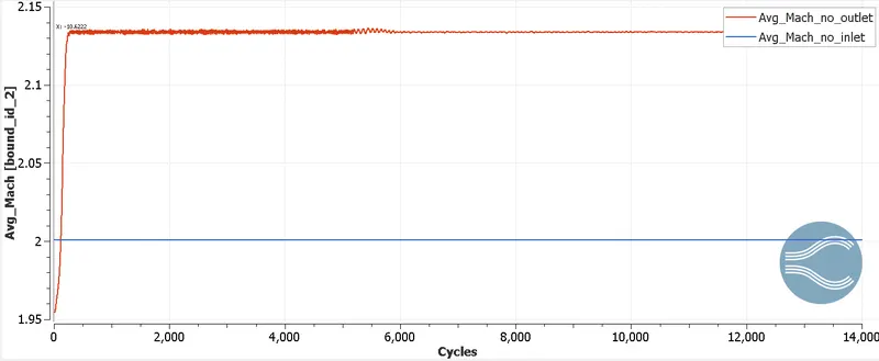
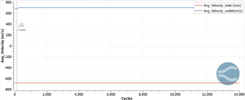
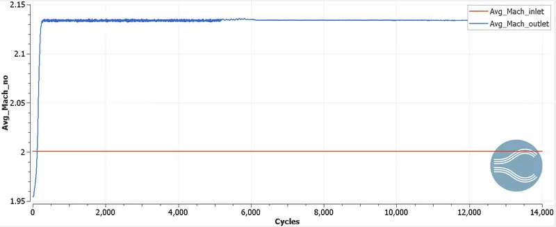
At 286.1 K, speed of sound in air is 340 m/sec. Hence Mach no, M = 680/340 = 2. Hence flow is supersonic and there is formation of schock wave.
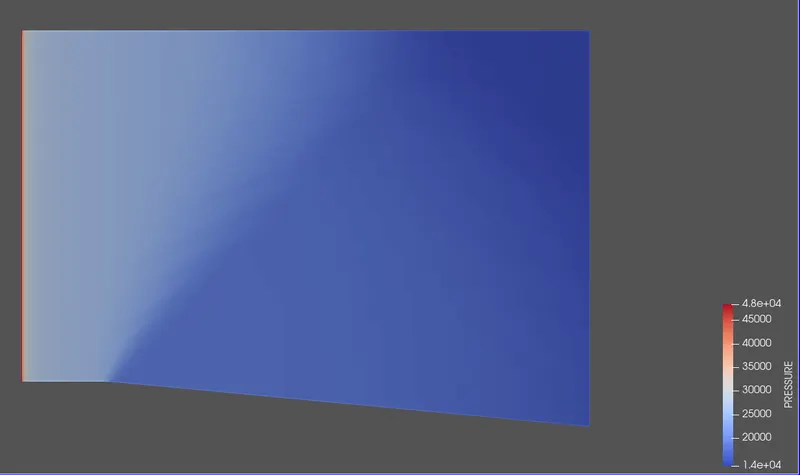
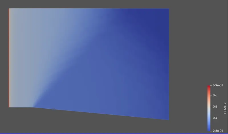
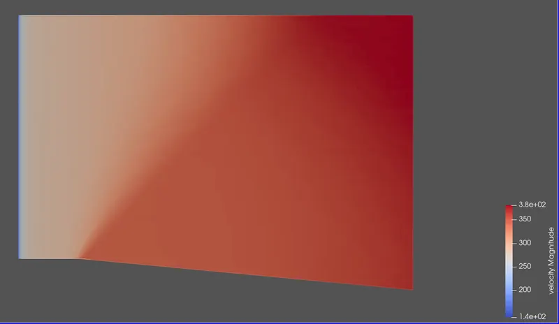
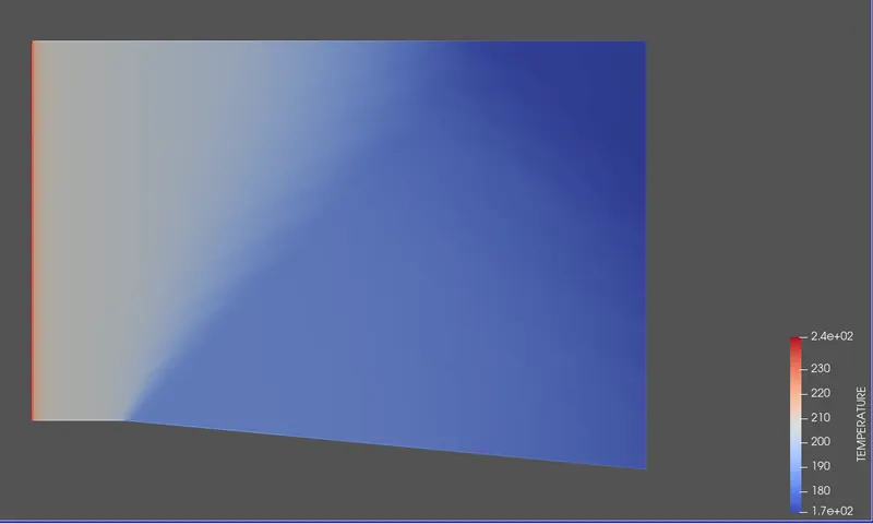
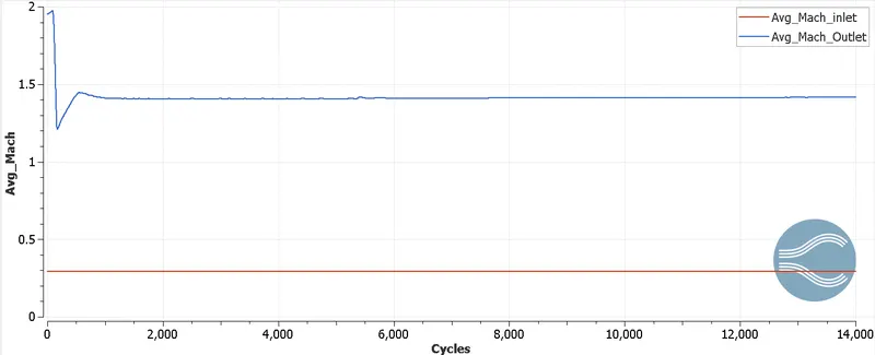
At 100 m/s inlet velocity, M = 100/340 = 0.29. Hence flow is sub-sonic and there is no shock wave formation.
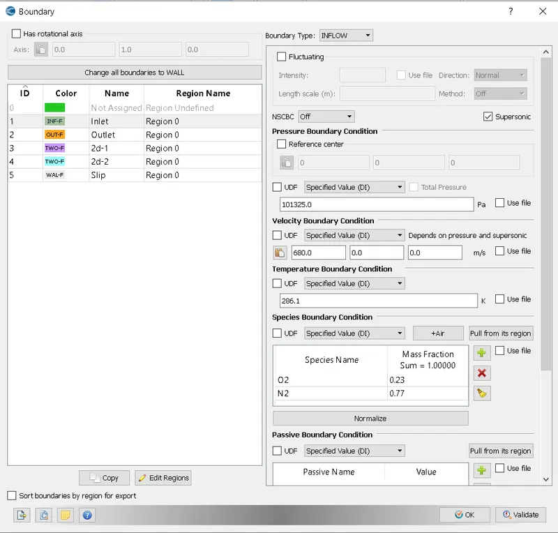
Outlet
Pressure: Zero normal gradient
Velocity: Zero normal gradient
Temperature: 300 K
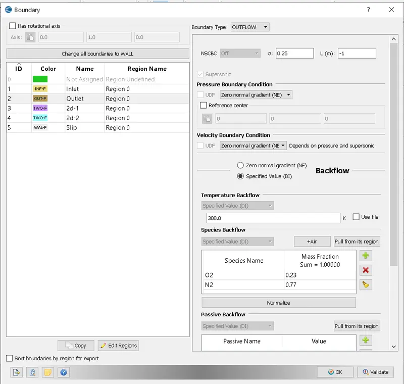
Walls: Slip boundary condition
Wall motion type: Stationary
Surafce movement: Fixed
Temperature: Zero normal gradient
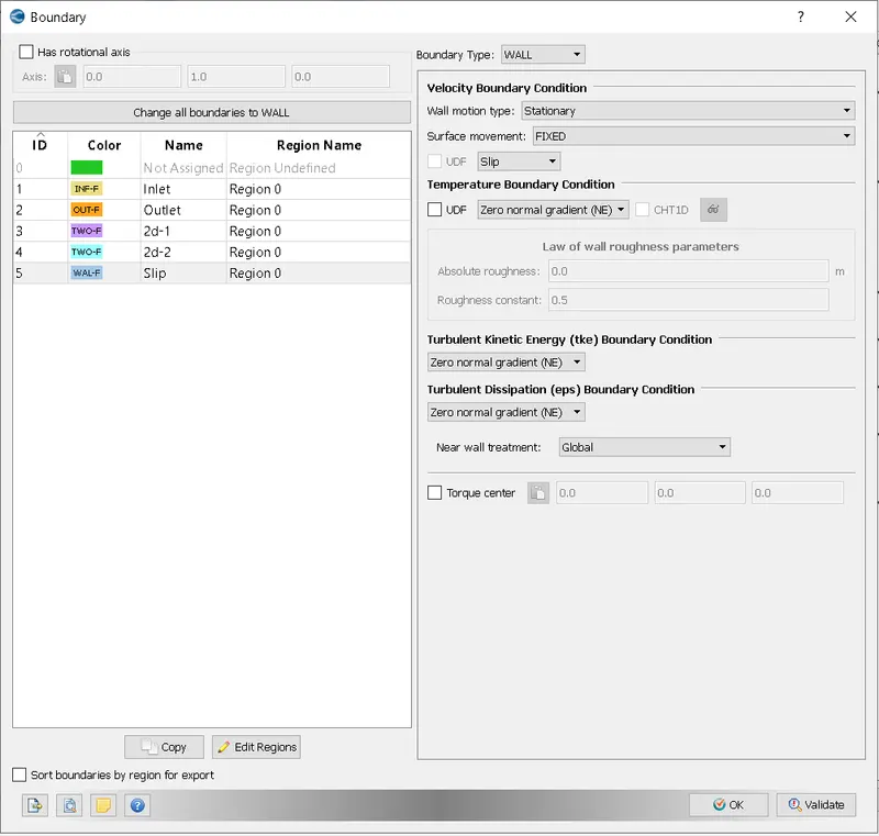
2D wall
Flow is considered to be 2D. Hence front and back wall is having boundary condition of 2D wall. Hence there is no flow along z-direction.
5) Regions and Initialisation
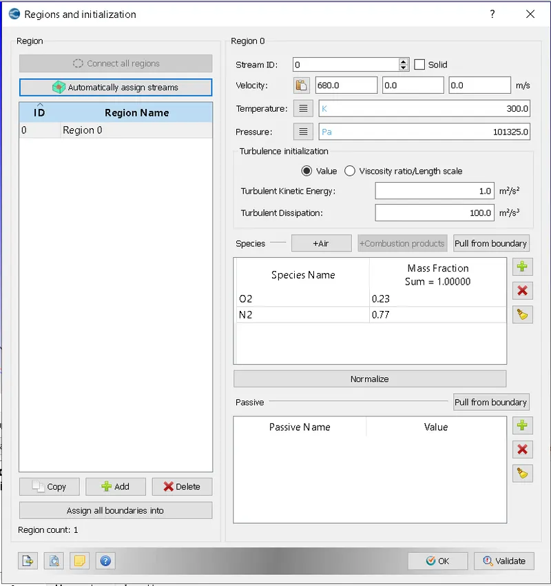
Region is initialised with temperture of 300 K and pressure of 101325 Pa
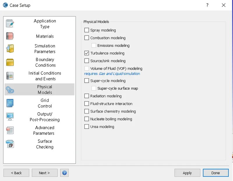
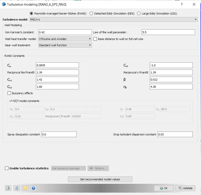
6) Physical models
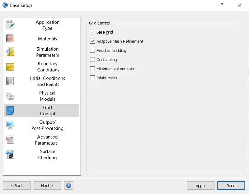
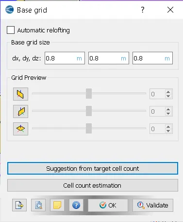
7) Grid controll
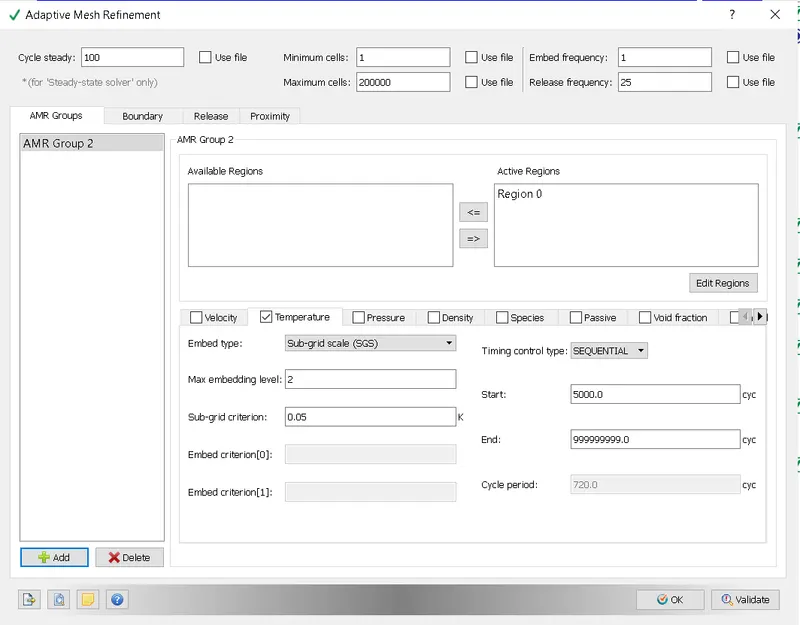
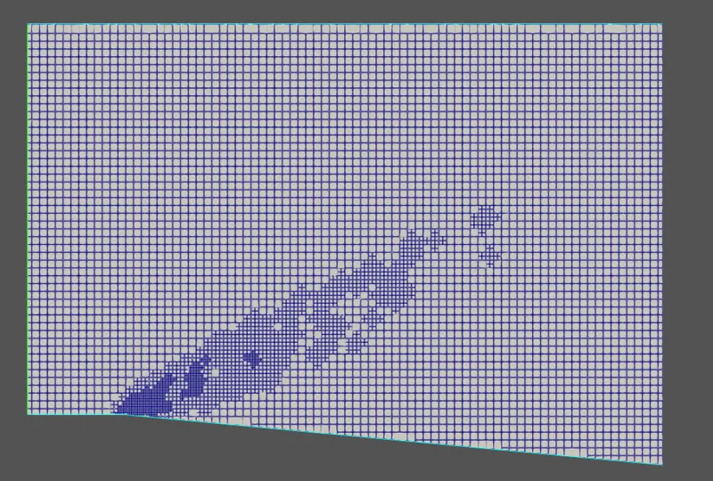
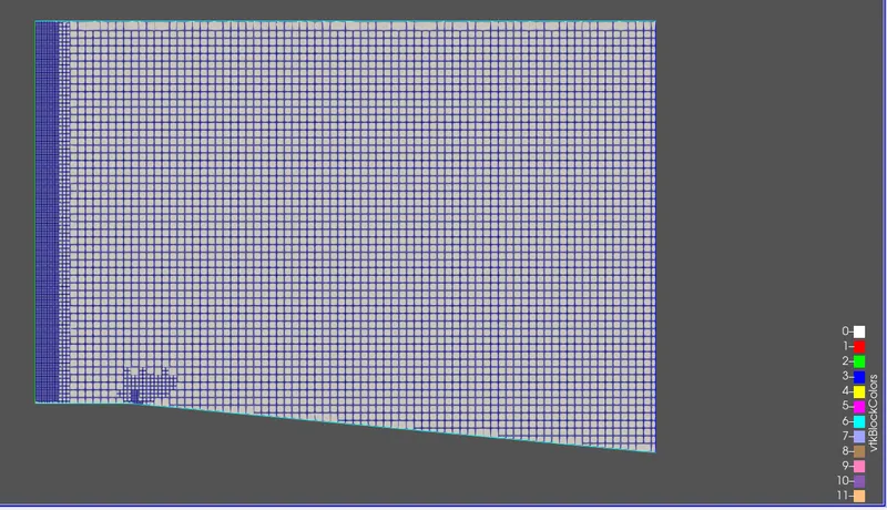
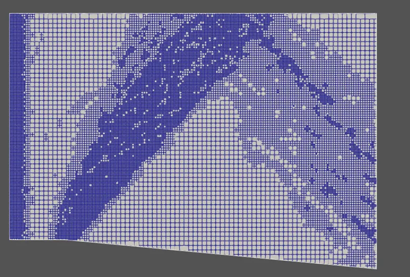
Adaptive mesh refinement (AMR) is used because in a region where shock wave forms, there is sudden change in flow properties like temperarure, pressure etc. To capture the flow physics correctly across shock wave, AMR is used which falicitates local refinement in mesh in the region where shock wave forms.
Results
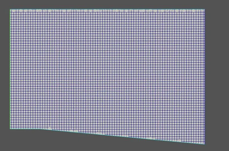
Initial mesh
1) Velocity 680 m/sec
a) SGS=0.05
Mesh at the end of simulation
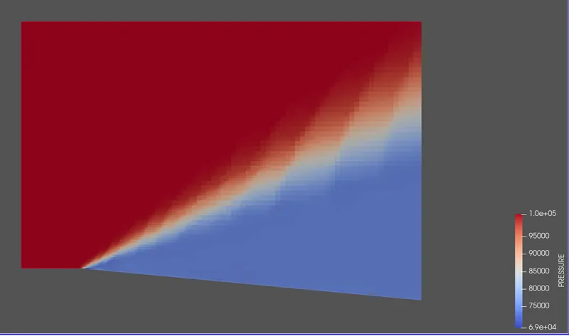
Pressure contour
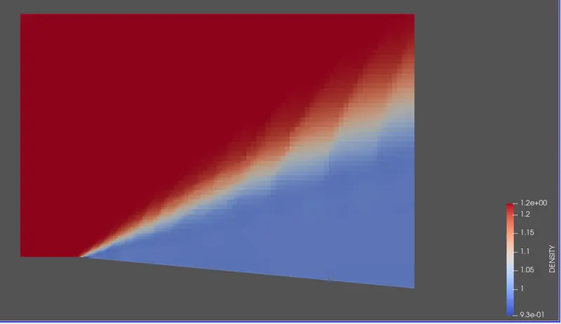
Density contour
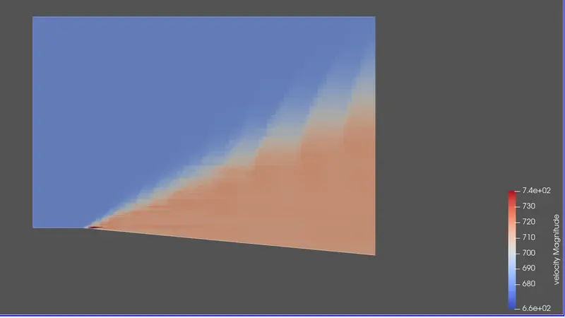
Velocity contour
Velocity animation: https://youtu.be/AeA22p6bEpc
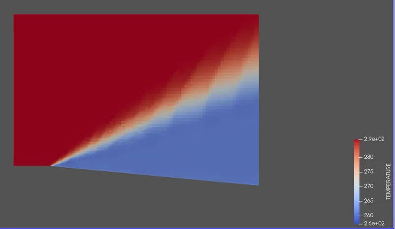
Temperature contour
Temperature animation: https://youtu.be/eop8oF1RTJE
Average Mach no
Average velocity
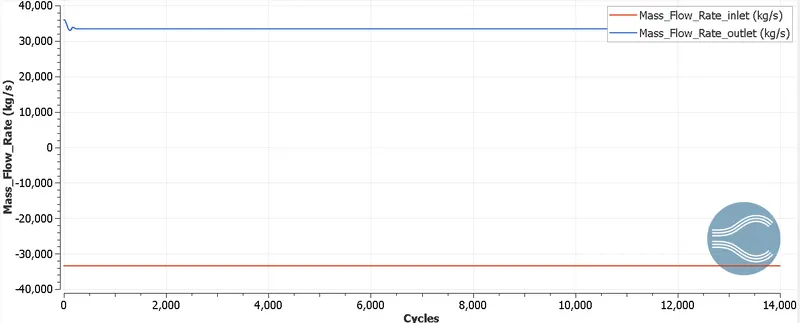
Mass flow rate
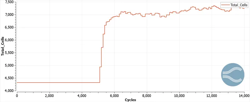
Total cells
b) SGS = 0.01
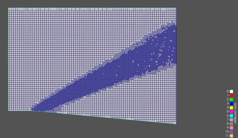
Mesh at the end of simulation
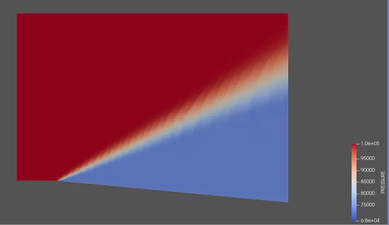
Pressure contour
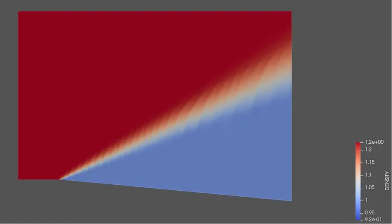
Density contour
Velocity contour
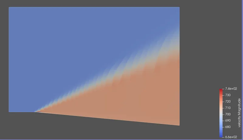
Velocity animation:https://youtu.be/TQMHtj5GYU0
Temperature contour
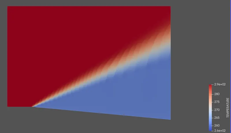
Temperature animation: https://youtu.be/dBunGpyOD4A
Average Mach no
Average velocity
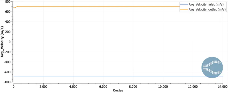
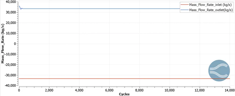
Average mass flow rate
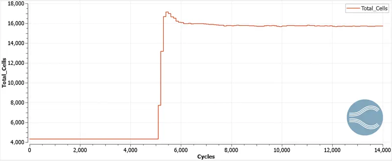
Total cells
2) Velocity 100 m/sec
a) SGS = 0.05
Mesh at the end of simulation
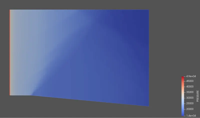
Pressure contour
Density contour
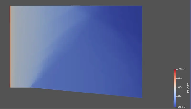
Velocity contour
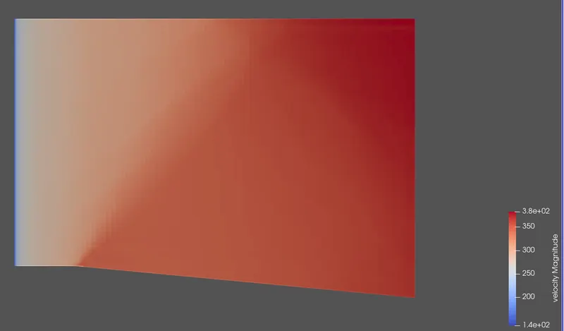
Velocity animation: https://youtu.be/sdZvw-xO3q8
Temperature contour
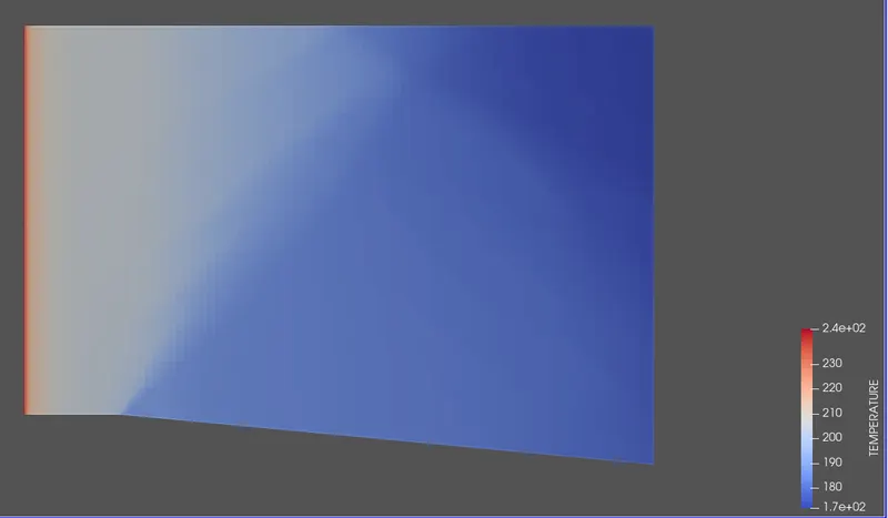
Temperature animation: https://youtu.be/HAH62zzdA24
Average Mach no
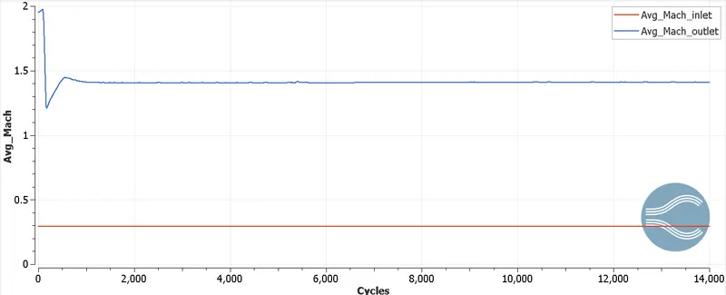
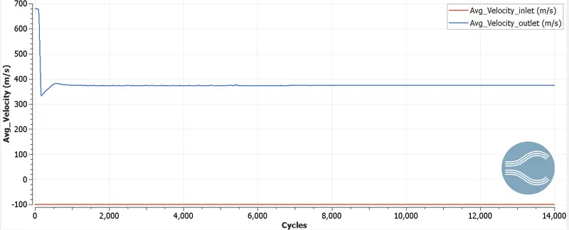
Average velocity
Average mass flow rate
Total cells
b) SGS = 0.01
Mesh at the end of simulation
Pressure contour
Density contour
Velocity contour
Velocity animation: https://youtu.be/GLYDnPhiU9g
Temperature contour
Temperature animation: https://youtu.be/2TRePL7UVkA
Average Mach no
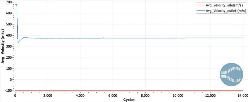
Average velocity
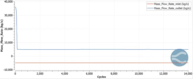
Average mass flow rate
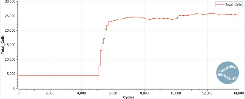
Total cells
Results and discussion
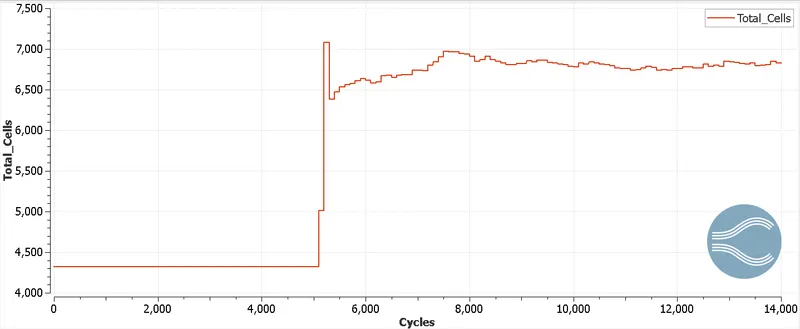
- As SGS parameter decreases, no of cells increses. Means lesser is the SGS parameter value, finer is the mesh (cell count is more for SGS 0.01 compared to SGS 0.05).
- For higher value of SGS parameter, the size refines mesh zone is less, but for less value of SGS parameter there is more mesh refinement.
- In supersonic flow, Prandtle mayor expansition fan is clearly visible and mesh refinement is also more as there is suddent change in flow properties like temperarure, pressure, velocity etc.
- For Subsonic flow, Prandtle mayor expansion fan is not clear visible and there is no suddent change in flow properties like temperarure, pressure, velocity etc.
- After 5000 cycles, cell count is incresasing in each case.
- In supersonic case (Velocity = 680 m/sec), there is formation of shock wave.
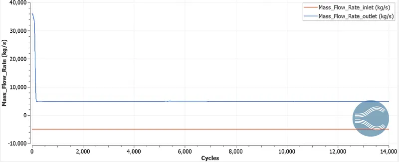
- Average mass flow rate at inlet and outlet is same. This ensures conservation of mass.