Week 7: Literature review - RANS derivation and analysis

Title: Reynolds Average Navier-Stokes equation (RANS) derivation and its Analysis

Aim: Introduction to Turbulance, turbulance modelling and RANS derivation.

Theory:

In fluid dynamics, turbulence or turbulent flow is fluid motion characterized by chaotic changes in pressure and flow velocity. It is in contrast to a laminar, which occurs when a fluid flows in parallel layers, with no disruption between those layers. In nature most of the flows are turbulent in nature except flow of some high viscous fluids.

Flow becomes turbulent at higher Reynolds no (Re) (which is ratio of Inertia force to Viscous force) where inertia forces dominates the viscous forces. Inertia forces tries to become flow to be turbulent on the other hand viscous forces tries to reduce turbulance in a fluid flow.

For flow through circular pipe, if Re<2000, flow is Laminar, if Re>4000, flow is turbulant and in between flow is in transition state.

Turbulent flows contains rotating structures called eddies. This eddies has wide range of length scales and time scales. Eddies can have length scales as large as system length scale such as a pipe diameter or length of flat plate or length scale may be very small.

Figure: Laminar and turbulant flows

In the turbulent flow, any turbulent quantity is expressed as a sum of mean quantity and fluctuating component of that quantity.

Figure: Fluctuation of flow quantity for Laminar and Turbulent flow.

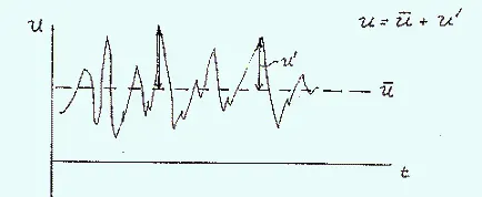
Figure: Variation of turbulant quantity in Laminar flow

Navier-Stokes equations for turbulant flows exhibit certain characteristics such as they are highly sensitive to initial conditions and they must adress wide lengths and time scales. Navier-Stokes equation cannot be applied as it is to the analysis of turbulent flows as in turbulent flows there is rapid fluctuation of turbulent quantity like pressure, velocity etc. And as in the turbulent flow, any turbulent quantity is expressed as a sum of mean quantity and fluctuating component of that quantity, Reylonds propesed the decomposition of any flow quantity into mean and fluctuating components. So in the Navier-Stokes equation, if we replace flow quantity with with its mean and fluctuating component, it is called as Reynolds decomposition or Reynolds averaging.

But resulting momentum equations after averaging has additional 9 stress components (called as Reynolds stresses), which are unknown. There are no explicite governing equations to find out this stresses. Hence to find out these stresses additional equations are needs to be solved. It is called as turbulance closure problem. The role of turbulance modelling is to find out this additional turbulent stresses.

Derivation of RANS is dicussed below.

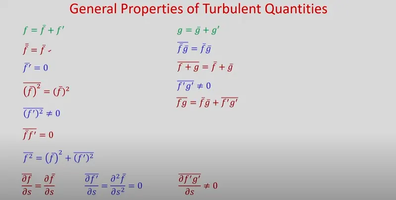
General properties of turbulent quantities

Let, f is a general flow property, which is summation of mean value and fluctuating component.

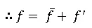
Where, f ̅ is mean component and `f^'`is fluctuating component.

Now average component can be found out as,

Therefore, time average of fluctuating component is always zero.

Now let,

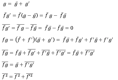
Above properties are shown in the below image

Navier-Stokes equation in conservative form for steady, incompressible flow with constant properties with usual notations

1) Continuity equation

`(∂u)/(∂x)+(∂v)/(∂y)+(∂w)/(∂z)=0`

2) X-momentum equation

``(∂u)/(∂t)+(∂(u u))/(∂x)+(∂(uv))/(∂y)+(∂(uw))/(∂z)=-1/ρ (∂p)/(∂x)+ν((∂^2 u)/(∂x^2 )+(∂^2 u)/(∂y^2 )+(∂^2 u)/(∂z^2 ))``

3) Y-momentum equation

`(∂v)/(∂t)+(∂(vu))/(∂x)+(∂(v v))/(∂y)+(∂(vw))/(∂z)=-1/ρ (∂p)/(∂x)+ν((∂^2 v)/(∂x^2 )+(∂^2 v)/(∂y^2 )+(∂^2 v)/(∂z^2 ))`

4) Z-momentum equation

`(∂w)/(∂t)+(∂(uw))/(∂x)+(∂(vw))/(∂y)+(∂(ww))/(∂z)=-1/ρ (∂p)/(∂x)+ν((∂^2 w)/(∂x^2 )+(∂^2 w)/(∂y^2 )+(∂^2 w)/(∂z^2 ))`

5) Energy equation

`(∂T)/(∂t)+(∂(uT))/(∂x)+(∂(vT))/(∂y)+(∂(wT))/(∂z)= α((∂^2 T)/(∂x^2 )+(∂^2 T)/(∂y^2 )+(∂^2 T)/(∂z^2 ))`

Reynolds averaging

First let us do Reynolds decomposition

`u= u ̅+u^'`, `v= v ̅+v^,`, `w= w ̅+w^'`, `p= p ̅+p^,` and `T= T ̅+T^'`--------------------1

Reynolds averaging of continuity equation

`(∂u)/(∂x)+(∂v)/(∂y)+(∂w)/(∂z)=0`

`(∂(u ̅+u^'))/(∂x)+(∂(v ̅+v^,))/(∂y)+(∂(w ̅+w^'))/(∂z)=0`

`(∂u ̅)/(∂x)+(∂v ̅)/(∂y)+(∂w ̅)/(∂z)+(∂u^')/(∂x)+(∂v^')/(∂y)+(∂w^')/(∂z)=0`

By taking time average

We know that, average of fluctuating component is zero. Hence

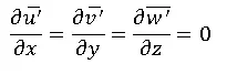
Hence after averaging continuity equation becomes,

`(∂u ̅)/(∂x)+(∂v ̅)/(∂y)+(∂w ̅)/(∂z)=0`

Therefore we can say that, time average velocity satisfies continuity equation.

Also we can get,

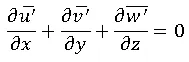
Means fluctuating component also satisfies continuity equation.

Reynolds averaging of x-momentum equation

`(∂u)/(∂t)+(∂(u u))/(∂x)+(∂(uv))/(∂y)+(∂(uw))/(∂z)=-1/ρ (∂p)/(∂x)+ν((∂^2 u)/(∂x^2 )+(∂^2 u)/(∂y^2 )+(∂^2 u)/(∂z^2 ))`

`(∂u)/(∂t)+(∂(u u))/(∂x)+(∂(uv))/(∂y)+(∂(uw))/(∂z)=-1/ρ (∂p)/(∂x)+ν∇^2 u`

Put equation 1 in above equation, we get

`(∂(u ̅+u^'))/(∂t)+(∂((u ̅+u^')(u ̅+u^')))/(∂x)+(∂((u ̅+u^')(v ̅+v^,)))/(∂y)+(∂((u ̅+u^')(w ̅+w^')))/(∂z)=-1/ρ (∂(p ̅+p^,))/(∂x)+ν∇^2 ( u ̅+u^')`

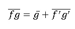
By taking time average of above equation and putting

, ,

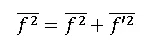On simplifying we will get,

Last 3 terms on right hand side inside square bracket are known as Reynolds apperent stress from momentum transfer from fluctuating velocity field.

Now, above equation can be written as,

Similarly procedure can be followed for Y and Z momentum equation

Reynolds averaging of Energy equation

`(∂T)/(∂t)+(∂(uT))/(∂x)+(∂(vT))/(∂y)+(∂(wT))/(∂z)= α((∂^2 T)/(∂x^2 )+(∂^2 T)/(∂y^2 )+(∂^2 T)/(∂z^2 ))`

`(∂T)/(∂t)+(∂(uT))/(∂x)+(∂(vT))/(∂y)+(∂(wT))/(∂z)= α∇^2 T`

Put `u= u ̅+u^'`, `v= v ̅+v^,`,`w= w ̅+w^'`and `T= T ̅+T^'`

`(∂(T ̅+T^'))/(∂t)+(∂((u ̅+u^')(T ̅+T^')))/(∂x)+(∂((v ̅+v^,)(T ̅+T^')))/(∂y)+(∂((w ̅+w^')(T ̅+T^')))/(∂z)= α∇^2 T`

By taking time average and properties of turbulance quantities, we get

On right side 3 quantities inside square bracket represents additional heat flux terms due to turbulent fluctuations/ turbulent motion.

Reynolds average Navier-Stokes equations

Continuity equation

`(∂u ̅)/(∂x)+(∂v ̅)/(∂y)+(∂w ̅)/(∂z)=0`

x-momentum equation

y-momentum equation

z-momentum equation

In tensor form, we can write momentum equations as,

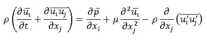
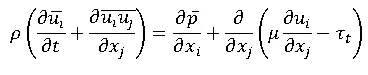
Above equations are known as Reynolds Average Navier-Stokes Equations (RANS)

Where, `τ_t` is turbulent stress or Reynolds stress.

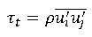
In tensor for, Reynolds stresses can be expressed as,

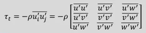
So, in above stress tensor six unknown terms are there, that needs to be find out. Above stresses are coming into picture due to turbulent fluctuations.

Energy equation

According to Boussinesq approximation,

Where, k is turbulant kinetic energy, `∂_ij = 1 if i=j`, otherwise `∂_ij =0`, `μ_t`is Eddy viscosity. `μ_t` is unknown in above equation

Now, total stress = Laminar stress + turbulent stres/Reynolds stress

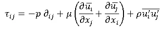
On rearranging,

Where,

`p_eff=(p+2/3 ρ k)`and `μ_eff=(μ+μ_t )`

Hence, in tensor form, Momentum equation becomes,

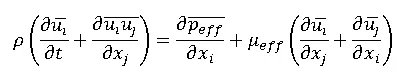
Eddy viscocity:

The turbulent transfer of momentum by eddied giving rise to an internal fluid friction in the same way as that of action of molecular viscocity in a transfer of momentum in laminar flow. Eddy viscocity is a measure of intenal fluid friction due to eddies in a turbulent flow. On the other hand molecular viscocity is measure of momentim transfer in Laminar flows.

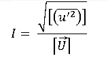
Turbulance Intensity:

The intensity of turbulence in a flow is described by the relative magnitude of the root mean square value of the fluctuating components with respect to the time average mean velocity. It is given by,

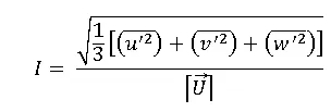
For Isotropic turbulance this is reduces to,

High turbulence case, `5≤I≤20`

Midium turbulence case, `1≤I≤5`

Turbulence case, `I<1`

Laminar Flow, I=0.

Closure problem in turbulance: Necessity of turbulance modelling

Turbulence modeling is the construction and use of a mathematical to predict the effects of turbualnce.

• In RANS, Reynolds stresses give additional unknowns but there are no explicite governing differential equations for that to solve for.
• Total unknowns = 3 Velocity components + 6 Reynolds stress terms + 1 pressure = 10.
• No of equations =4 (1 Continuity + 3 Momentum)
• As No. of unknowns are > No. of equations, the problem is indeterminate. One needs to close the problem to obtain a solution. This is known as closure problem in turbualnce.
• The turbulance modelling tries to represent the reynolds stresses in terms of time-average velocity components.
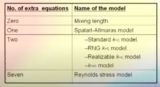
• The common turbulance models are classified on the basis of the number of additional transport equations that need to be solved along with RANS equations.

Turbulance model may be

1) Eddy viscocity model

2) Reynolds stress transport model

Following are the some of the turbulance models according to no. of additional governing equations to be solved.