Week 7 - Minor Project

Creating a domain for compressible and incompressible flow over a NACA 0012 airfoil

(i) We need to import the airfoil data from the below-mentioned URL,

http://www.basiliscus.com/ProaSections/AppendixD/TableD1.txt

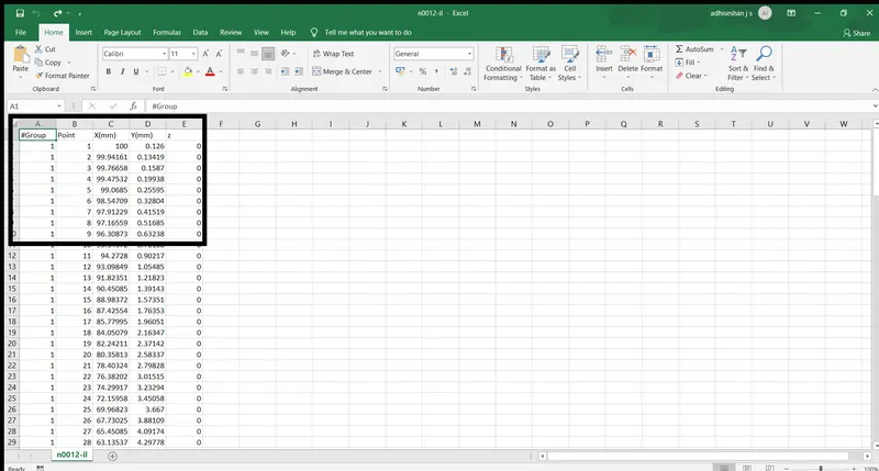
(ii) After downloading the data, we want to edit manually the 3 dimension co-ordinates and also the point numbering in an Excel file as shown below,

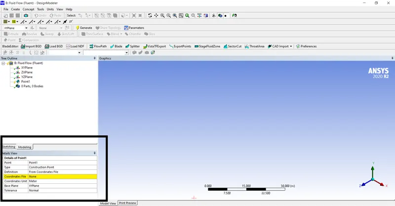
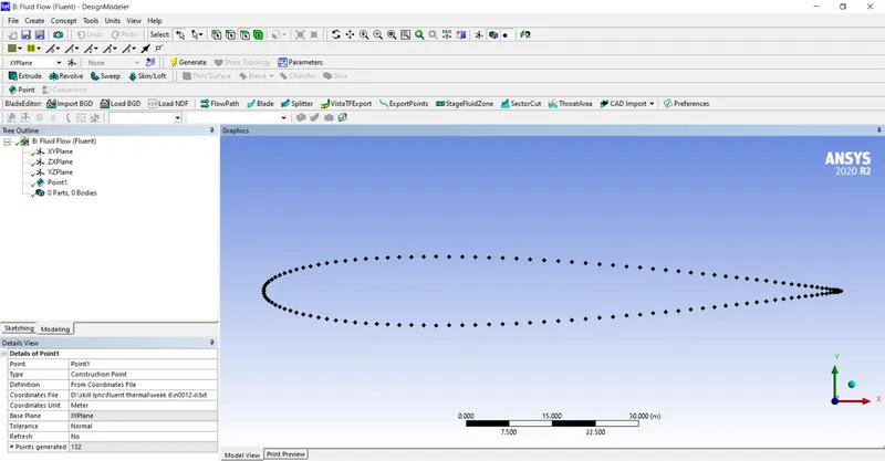
(iii) Then we have to save the file to .txt format, afterward in Design Modeler Import the text file using Points Feature as shown below,

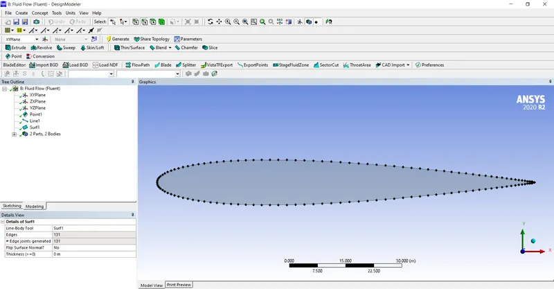
(iv) After creating Points we have created edges using the edges from points option as shown below,

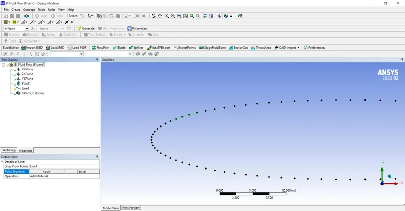
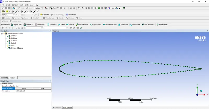
Generate the edges and use surface from edges feature to create the airfoil surface.

(v) After this we will see how to create the domain mentioned in the video,

First, we need to create the lines according to the dimensions given for the domain.

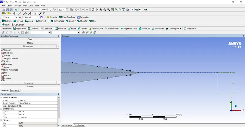
Add dimensions to the horizontal and vertical Lines

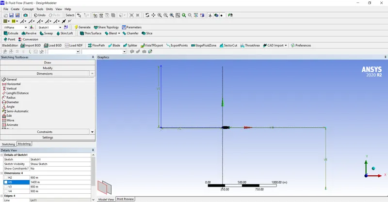
Create a two-point rectangle using the created lines an points.

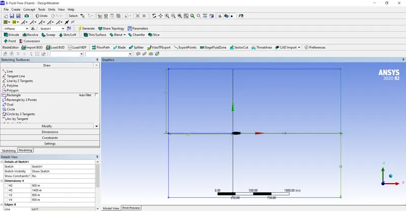
Delete the exceed lines that are not required for the domain using the trim option.

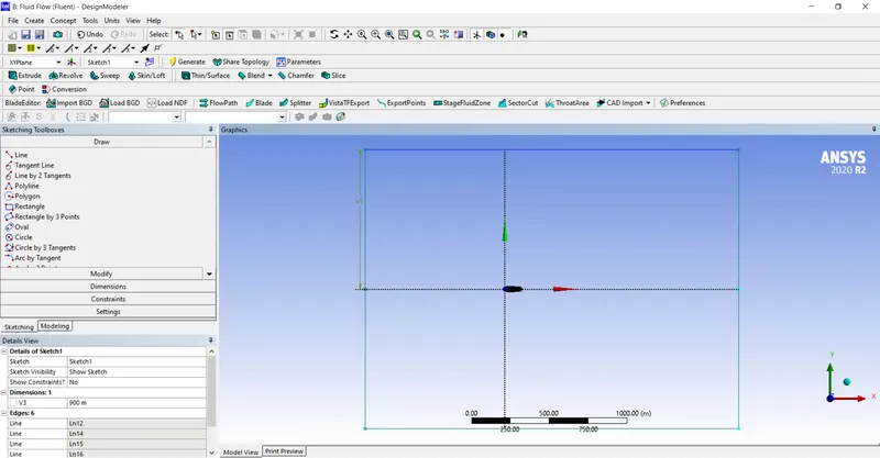
Create a three-point arc in the inlet section and cut the unwanted lines.

Create a plane and delete the extra airfoil plane using Boolean operation as shown below,

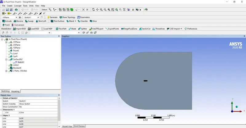
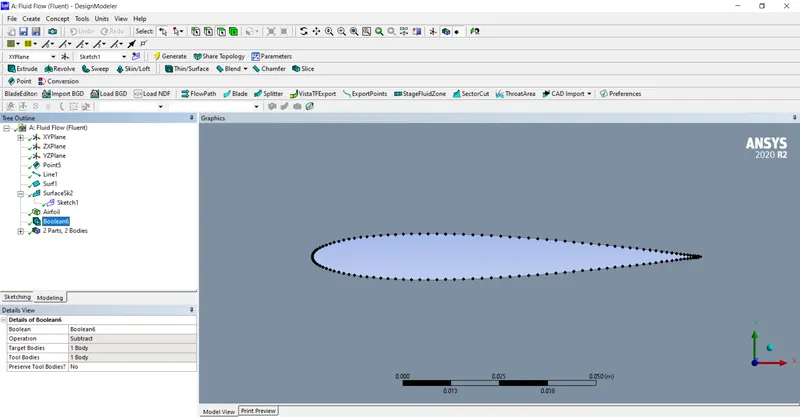
(ii) Meshing:

Base Mesh Size = 150m :

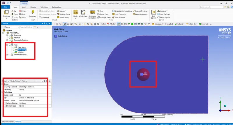
Step 1: Body Sizing

• Insert sizing in the mesh and add body sizing feature
• Select the body which is shown below, and use the sphere of influence type and provide the required dimension.
• We can refine the mesh size as we want. mesh size=0.5mm.

Step 2: Face Sizing

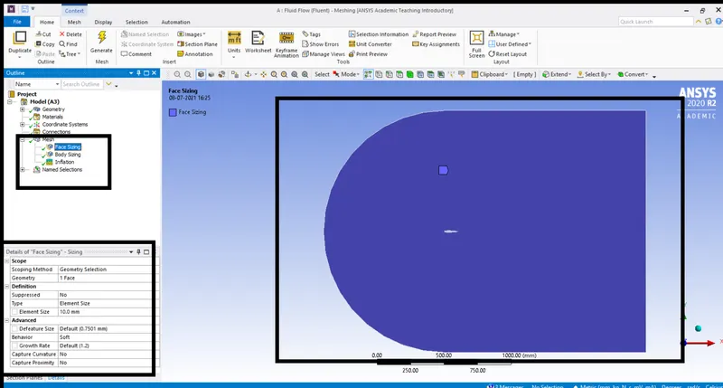
• Insert sizing in the mesh and add face sizing feature
• Select the face which is shown below, and give element size as 0.2m.
• We can refine the mesh size as we want. mesh size=10mm.

Step 3: Inflation

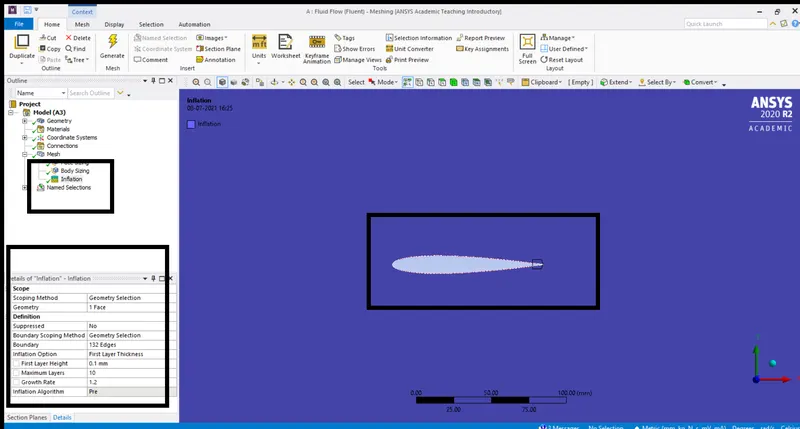
• Insert sizing in the mesh and add inflation feature
• Select the boundary which is shown below, and give the first layer height as calculated and, maximum layer thickness.
• We can refine the mesh size as we want.

Results:

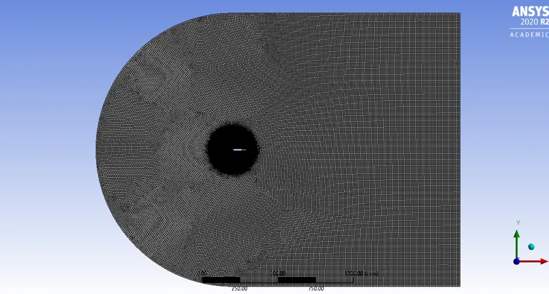
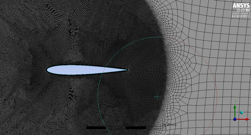
Total Mesh Domain

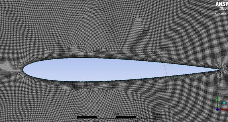
Boundary Meshing

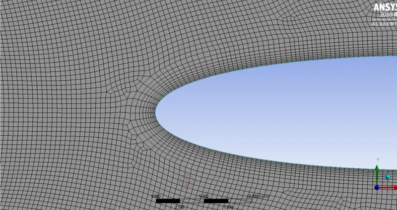
Inflation Layer

Pre-processing and solver setting

Incompressible cases:

Case 1: (Angle of Attack = 0)

The next step in the simulation after generating the meshing is to set up the physical properties for the case.

• Type of solver: Pressure-based
• Simulation method: Steady-state simulation
• Turbulent Model: k-omega standard
• Material properties of the fluid (Air)

Density: 2.131 kg/m3

Cp (Specific heat): 1006.43 J/kg-k

Thermal Conductivity: 0.0242 w/m-k

Viscosity: 1.7894e-05 kg/m-s

• Inlet velocity: X velocity = 52.15 m/s, Y velocity = 0 m/s
• Inlet Temperature: 300 K
• Outlet: Pressure type, 0-gauge pressure.
• Walls: wall type with no-slip

Results

After setting up a case and providing appropriate initial and boundary conditions, the number of simulations are performed Airfoil, mainly for the comparison of results from different angles of attacks.

Results of Case 1

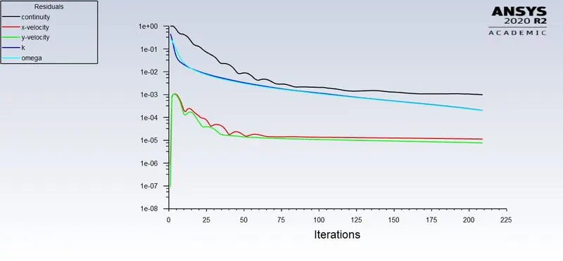
Residuals

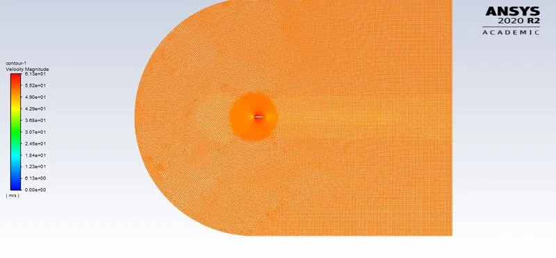
Velocity Contour

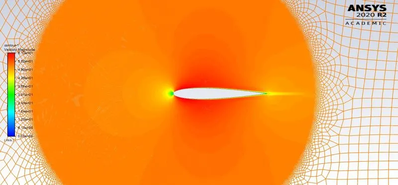
Close Look at the velocity contour

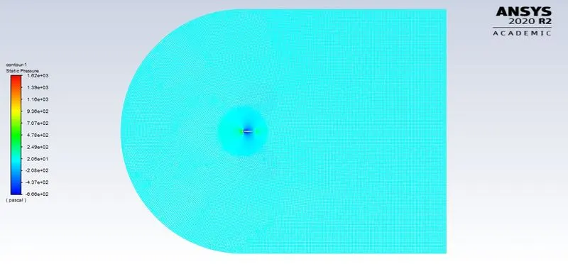
Pressure Contour

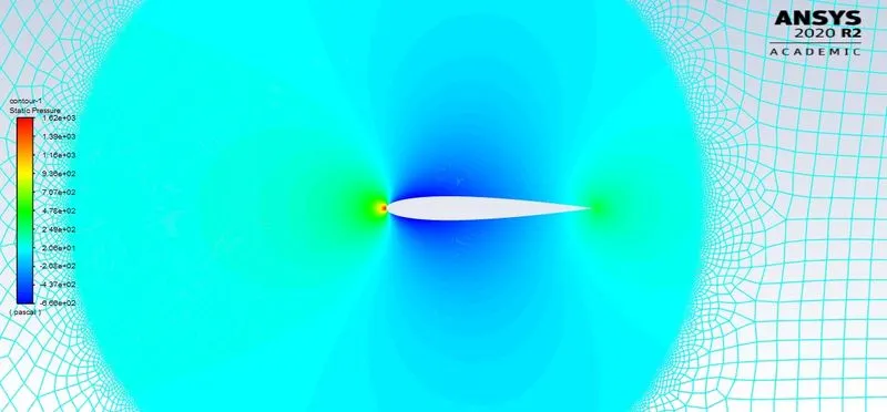
Close Look at the pressure contour

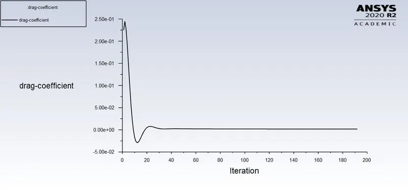
Drag Coefficient

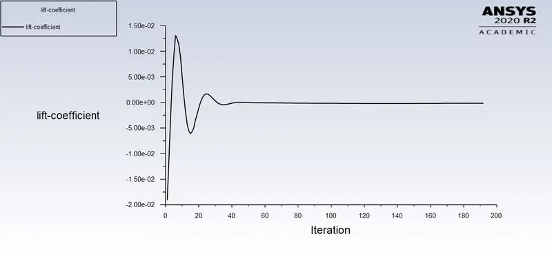
Lift Coefficient

Case 2: (Angle of Attack = 5)

The next step in the simulation after generating the meshing is to set up the physical properties for the case.

• Type of solver: Pressure-based
• Simulation method: Steady-state simulation
• Turbulent Model: k-omega standard
• Material properties of the fluid (Air)

Density: 2.131 kg/m3

Cp (Specific heat): 1006.43 J/kg-k

Thermal Conductivity: 0.0242 w/m-k

Viscosity: 1.7894e-05 kg/m-s

• Inlet velocity: X velocity = 51.802 m/s, Y velocity = 4.53 m/s
• Inlet Temperature: 300 K
• Outlet: Pressure type, 0-gauge pressure.
• Walls: wall type with no-slip

Results

After setting up a case and providing appropriate initial and boundary conditions, the number of simulations is performed Airfoil, mainly for the comparison of results from different angles of attacks.

Results of Case 2

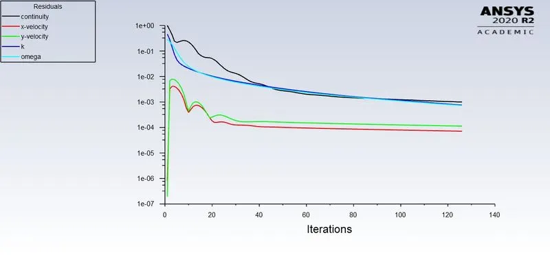
Residuals

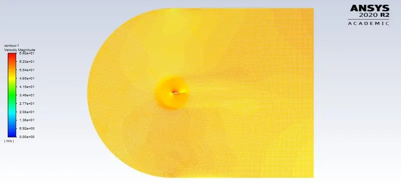
Velocity Contour

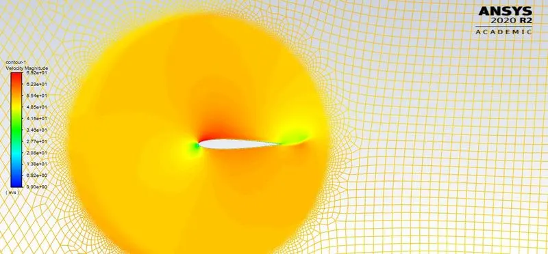
Close Look at the velocity contour

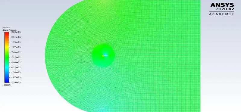
Pressure Contour

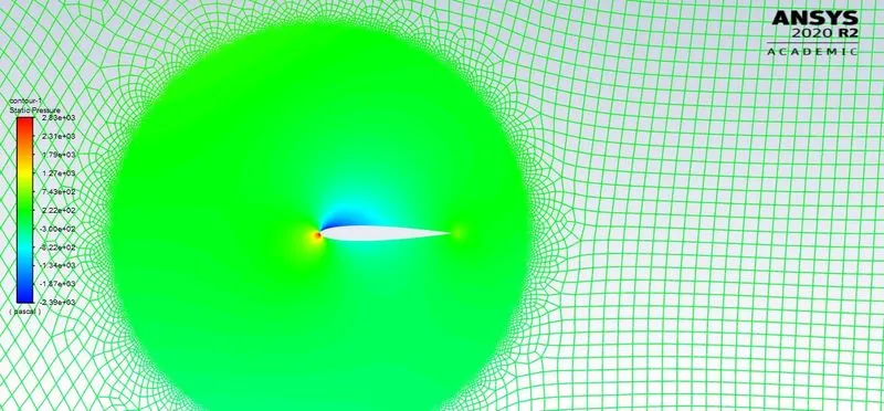
Close Look at the pressure contour

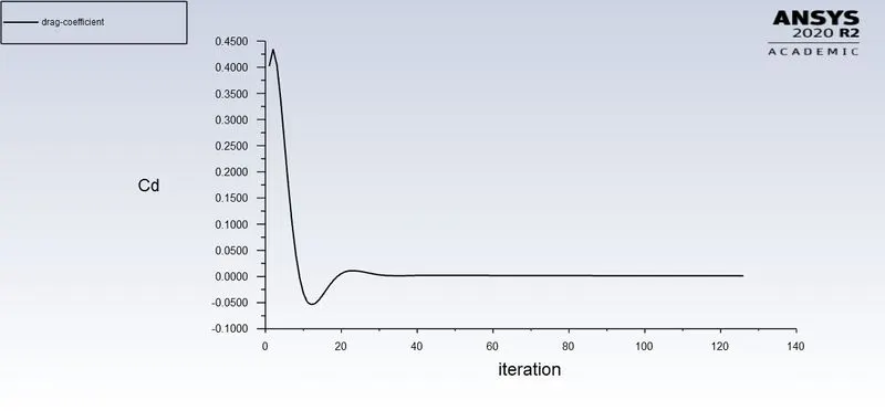
Drag Coefficient

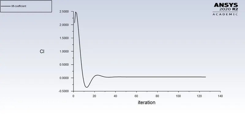
Lift Coefficient

Case 3: (Angle of Attack = 10)

The next step in the simulation after generating the meshing is to set up the physical properties for the case.

• Type of solver: Pressure-based
• Simulation method: Steady-state simulation
• Turbulent Model: k-omega standard
• Material properties of the fluid (Air)

Density: 2.131 kg/m3

Cp (Specific heat): 1006.43 J/kg-k

Thermal Conductivity: 0.0242 w/m-k

Viscosity: 1.7894e-05 kg/m-s

• Inlet velocity: X velocity = 51.21 m/s, Y velocity = 9.029 m/s
• Inlet Temperature: 300 K
• Outlet: Pressure type, 0-gauge pressure.
• Walls: wall type with no-slip

Results

After setting up a case and providing appropriate initial and boundary conditions, the number of simulations is performed Airfoil, mainly for the comparison of results from different angles of attacks.

Results of Case 3

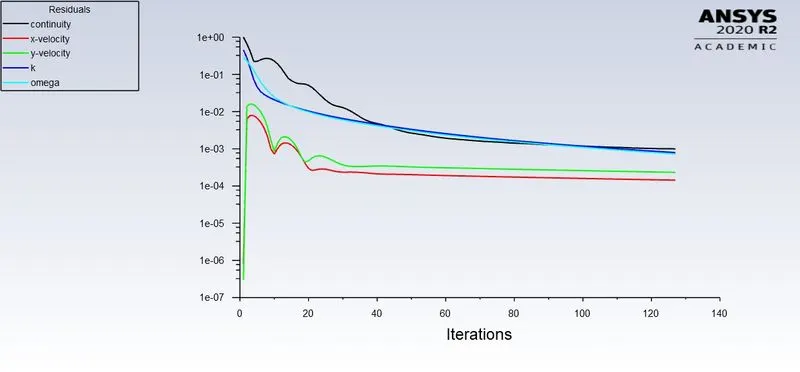
Residuals

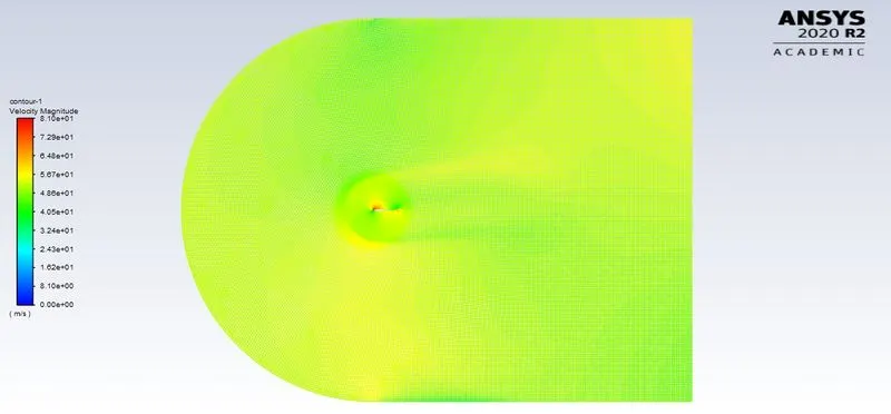
Velocity Contour

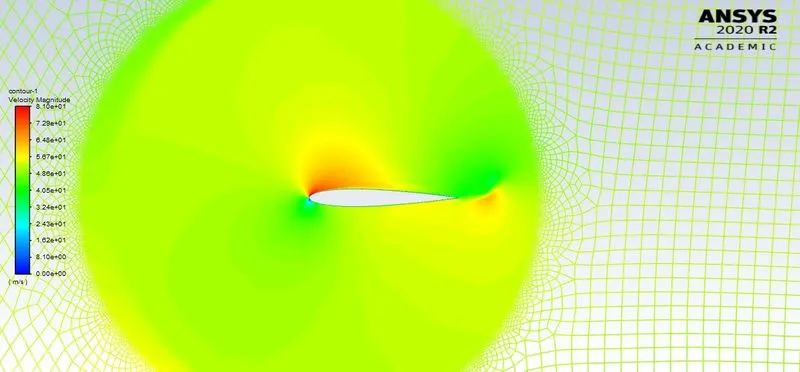
Close Look at the velocity contour

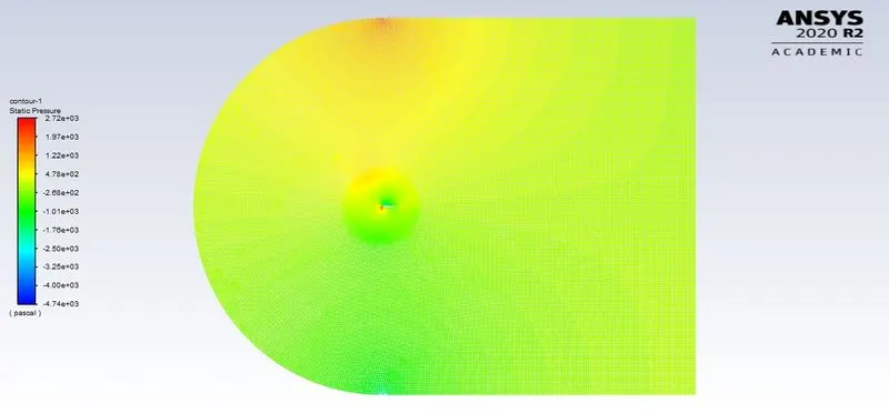
Pressure Contour

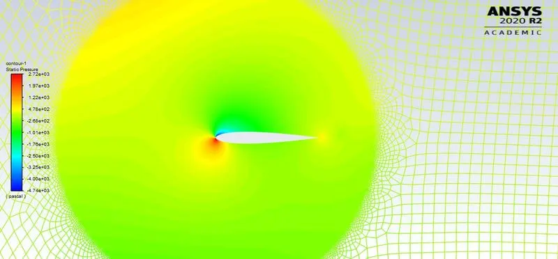
Close Look at the pressure contour

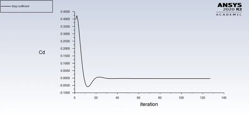
Drag Coefficient

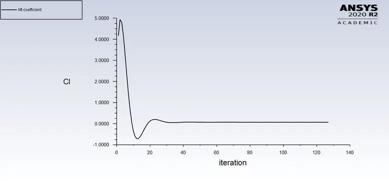
Lift Coefficient

Case 4: (Angle of Attack = 15)

The next step in the simulation after generating the meshing is to set up the physical properties for the case.

• Type of solver: Pressure-based
• Simulation method: Steady-state simulation
• Turbulent Model: k-omega standard
• Material properties of the fluid (Air)

Density: 2.131 kg/m3

Cp (Specific heat): 1006.43 J/kg-k

Thermal Conductivity: 0.0242 w/m-k

Viscosity: 1.7894e-05 kg/m-s

• Inlet velocity: X velocity = 50.22 m/s, Y velocity = 13.45 m/s
• Inlet Temperature: 300 K
• Outlet: Pressure type, 0-gauge pressure.
• Walls: wall type with no-slip

Results

After setting up a case and providing appropriate initial and boundary conditions, the number of simulations is performed Airfoil, mainly for the comparison of results from different angles of attacks.

Results of Case 4

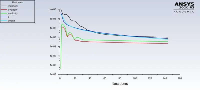
Residuals

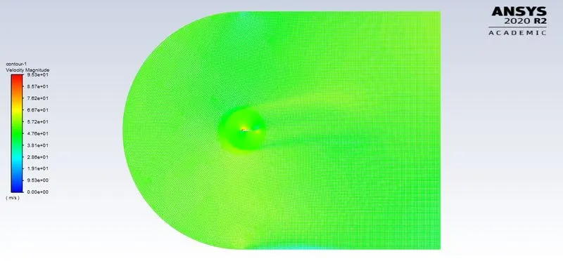
Velocity Contour

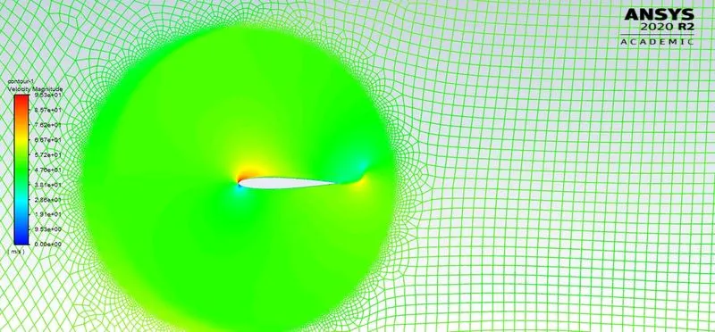
Close Look at the velocity contour

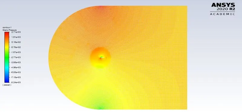
Pressure Contour

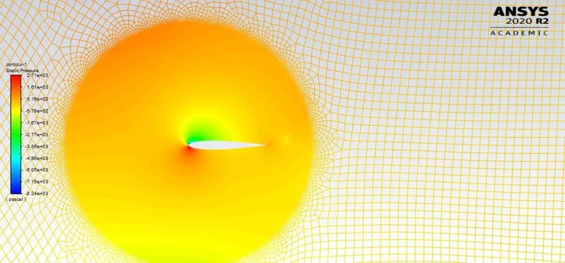
Close Look at the pressure contour

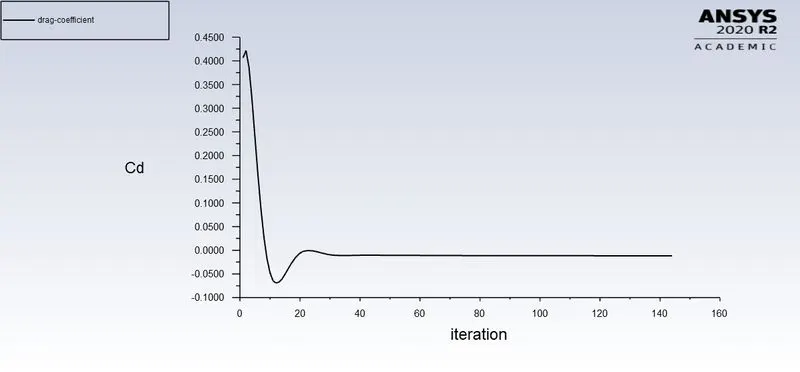
Drag Coefficient

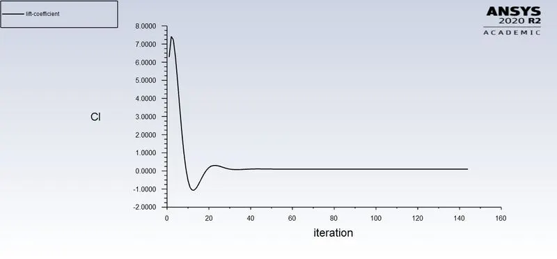
Lift Coefficient

Compressible cases:

Case 1: (Angle of Attack = 0)

The next step in the simulation after generating the meshing is to set up the physical properties for the case.

• Type of solver: Density-based
• Simulation method: Steady-state simulation
• Turbulent Model: k-omega standard
• Material properties of the fluid (Air)

Density: 1.225 kg/m3

Cp (Specific heat): 1006.43 J/kg-k

Thermal Conductivity: 0.0242 w/m-k

Viscosity: 1.7894e-05 kg/m-s

• Inlet velocity: X velocity = 272 m/s, Y velocity = 0 m/s
• Inlet Temperature: 300 K
• Outlet: Pressure type, 0-gauge pressure.
• Walls: wall type with no-slip

Results

After setting up a case and providing appropriate initial and boundary conditions, the number of simulations are performed Airfoil, mainly for the comparison of results from different angles of attacks.

Results of Case 1

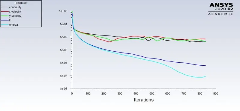
Residuals

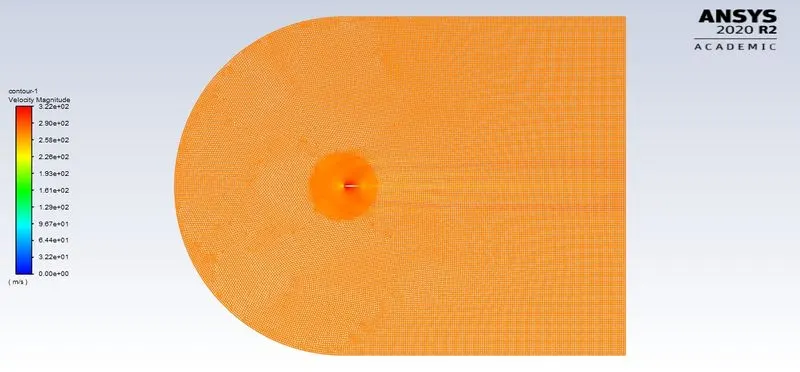
Velocity Contour

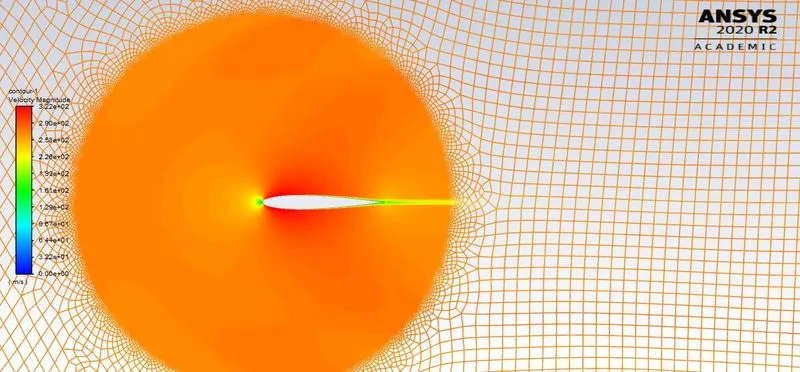
Close Look at the velocity contour

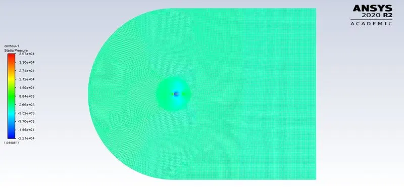
Pressure Contour

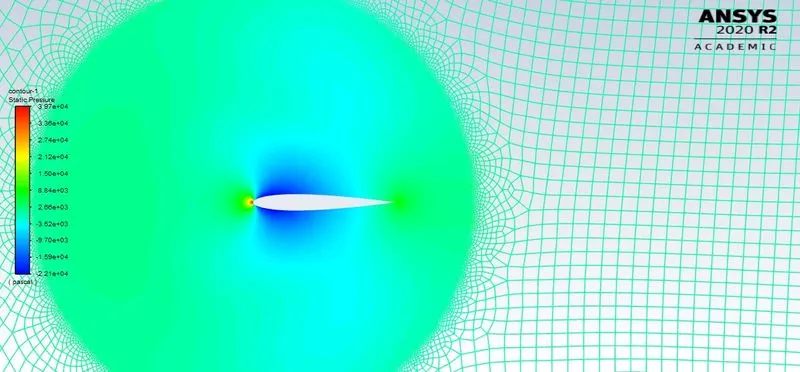
Close Look at the pressure contour

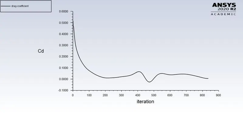
Drag Coefficient

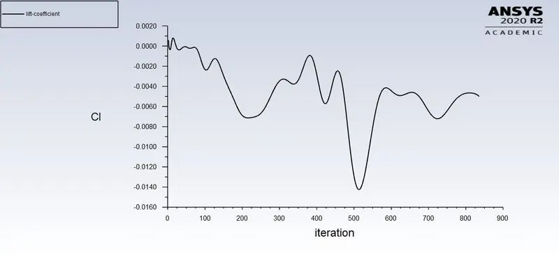
Lift Coefficient

Case 2: (Angle of Attack = 5)

The next step in the simulation after generating the meshing is to set up the physical properties for the case.

• Type of solver: Density-based
• Simulation method: Steady-state simulation
• Turbulent Model: k-omega standard
• Material properties of the fluid (Air)

Density: 1.225 kg/m3

Cp (Specific heat): 1006.43 J/kg-k

Thermal Conductivity: 0.0242 w/m-k

Viscosity: 1.7894e-05 kg/m-s

• Inlet velocity: X velocity = 270.964 m/s, Y velocity = 23.706 m/s
• Inlet Temperature: 300 K
• Outlet: Pressure type, 0-gauge pressure.
• Walls: wall type with no-slip

Results

After setting up a case and providing appropriate initial and boundary conditions, the number of simulations are performed Airfoil, mainly for the comparison of results from different angles of attacks.

Results of Case 2

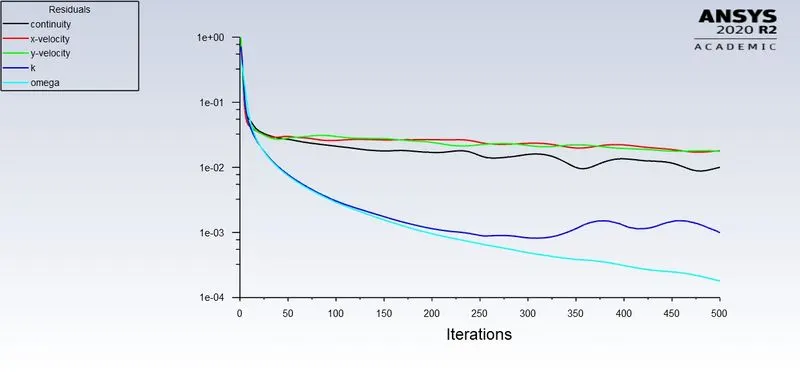
Residuals

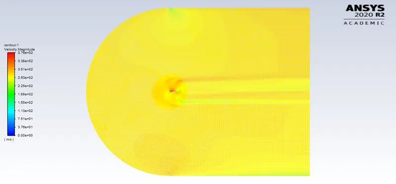
Velocity Contour

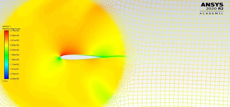
Close Look at the velocity contour

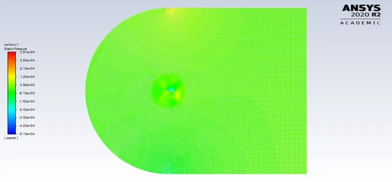
Pressure Contour

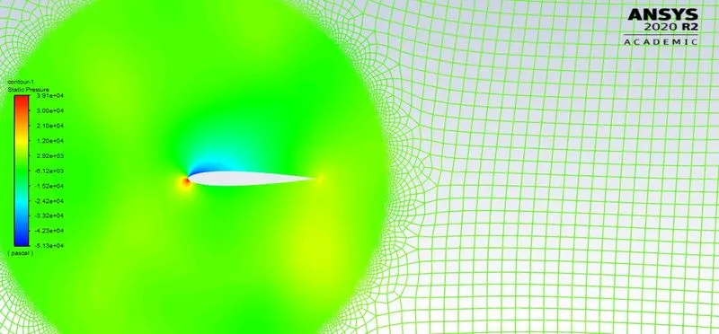
Close Look at the pressure contour

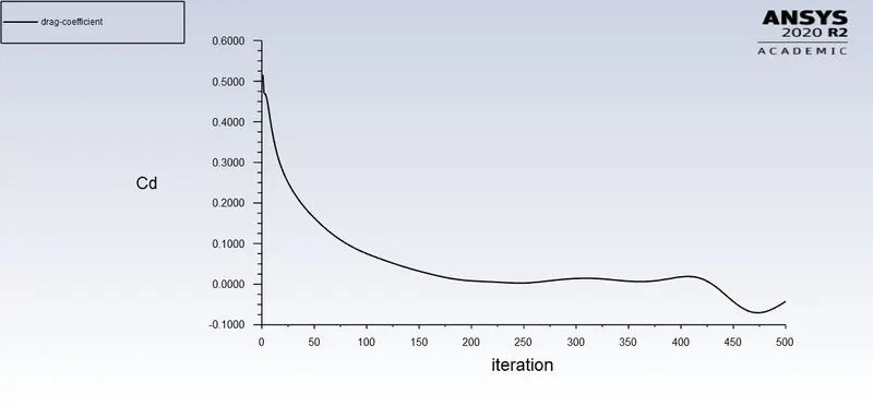
Drag Coefficient

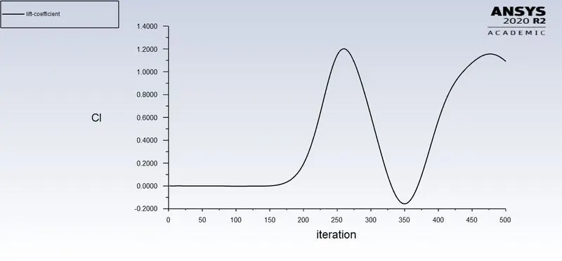
Lift Coefficient

Case 3: (Angle of Attack = 10)

The next step in the simulation after generating the meshing is to set up the physical properties for the case.

• Type of solver: Density-based
• Simulation method: Steady-state simulation
• Turbulent Model: k-omega standard
• Material properties of the fluid (Air)

Density: 1.225 kg/m3

Cp (Specific heat): 1006.43 J/kg-k

Thermal Conductivity: 0.0242 w/m-k

Viscosity: 1.7894e-05 kg/m-s

• Inlet velocity: X velocity = 267.867 m/s, Y velocity = 47.232 m/s
• Inlet Temperature: 300 K
• Outlet: Pressure type, 0-gauge pressure.
• Walls: wall type with no-slip

Results

After setting up a case and providing appropriate initial and boundary conditions, the number of simulations is performed Airfoil, mainly for the comparison of results from different angles of attacks.

Results of Case 3

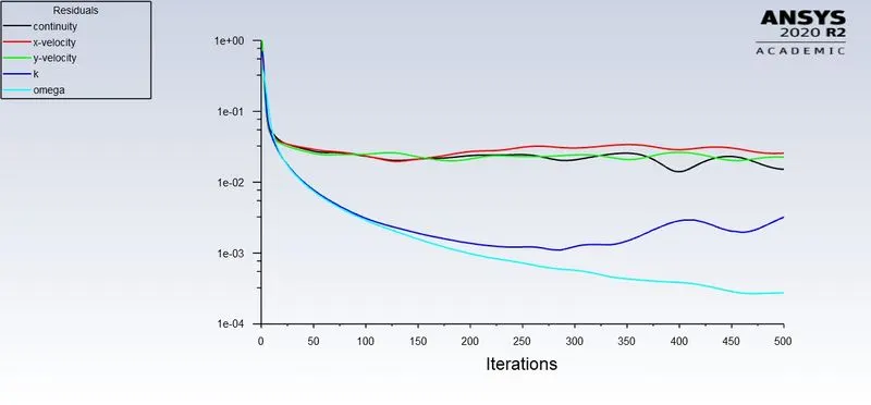
Residuals

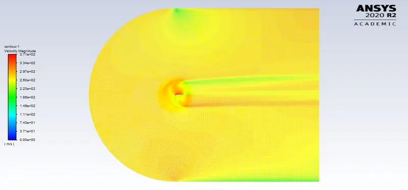
Velocity Contour

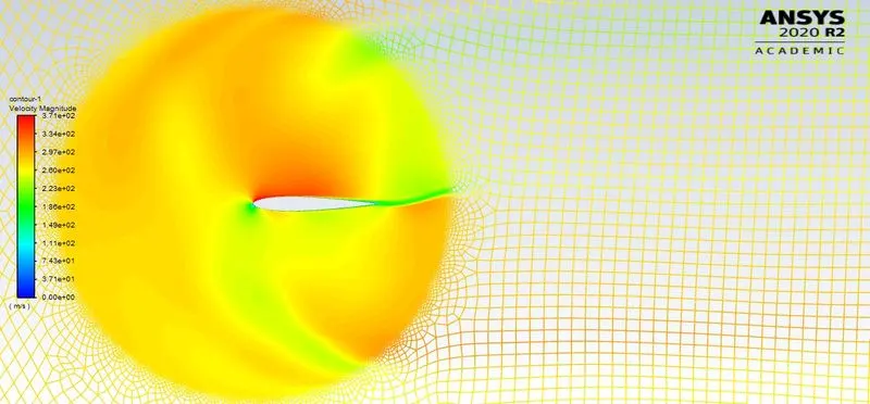
Close Look at the velocity contour

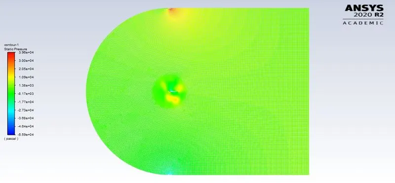
Pressure Contour

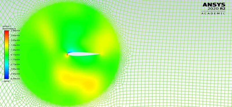
Close Look at the pressure contour

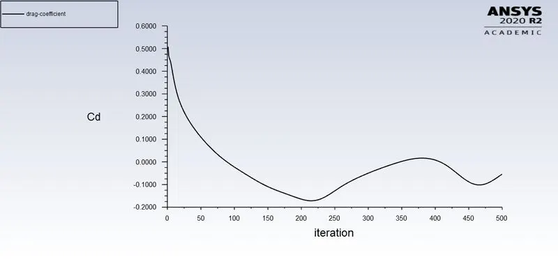
Drag Coefficient

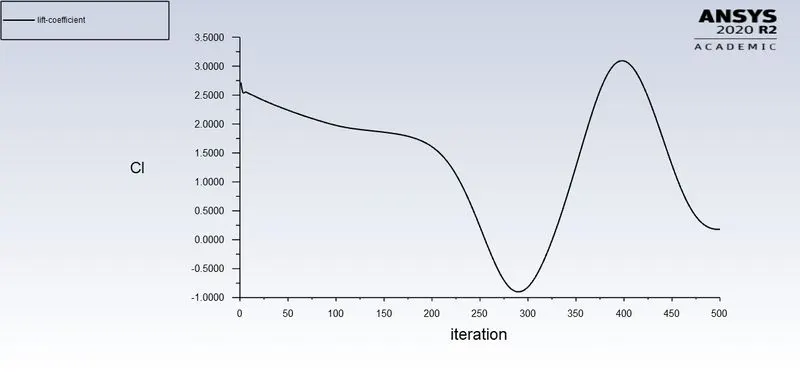
Lift Coefficient

Case 4: (Angle of Attack = 15)

The next step in the simulation after generating the meshing is to set up the physical properties for the case.

• Type of solver: Density-based
• Simulation method: Steady-state simulation
• Turbulent Model: k-omega standard
• Material properties of the fluid (Air)

Density: 1.225 kg/m3

Cp (Specific heat): 1006.43 J/kg-k

Thermal Conductivity: 0.0242 w/m-k

Viscosity: 1.7894e-05 kg/m-s

• Inlet velocity: X velocity = 262.731 m/s, Y velocity = 70.398 m/s
• Inlet Temperature: 300 K
• Outlet: Pressure type, 0-gauge pressure.
• Walls: wall type with no-slip

Results

After setting up a case and providing appropriate initial and boundary conditions, the number of simulations is performed Airfoil, mainly for the comparison of results from different angles of attacks.

Results of Case 4

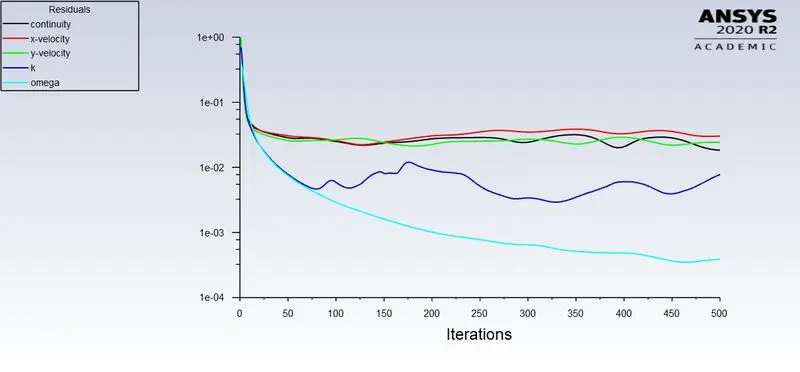
Residuals

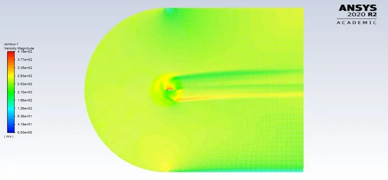
Velocity Contour

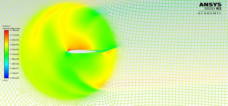
Close Look at the velocity contour

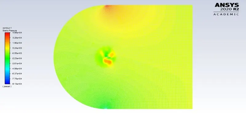
Pressure Contour

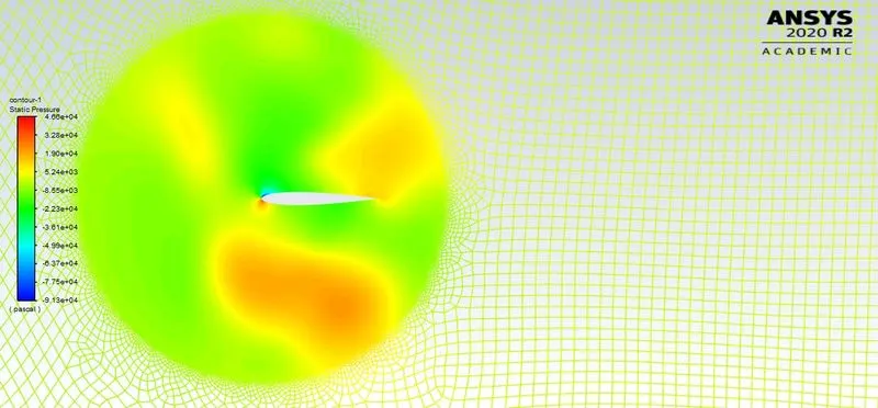
Close Look at the pressure contour

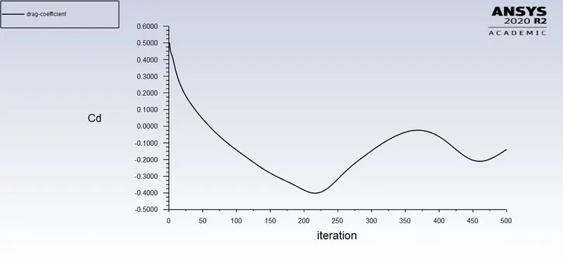
Drag Coefficient

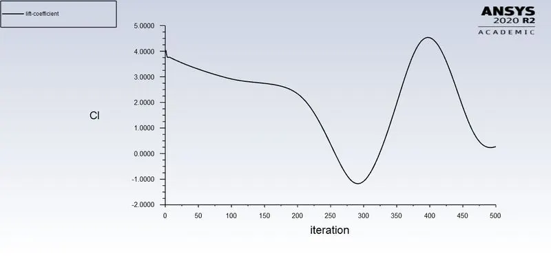
Lift Coefficient