Project Steady state simulation of flow over a throttle body
Steady state simulation of flow over a throttle body
Aim:
The main objective of this project is to set up the case to perform simulation of steady-state flow over a Throttle valve when it is fully open and post-processing the result using ParaView.
Introduction:
The report contains a detailed description of the steady-state flow simulation over a Throttle valve using converge CFD software, solving it using CYGWIN and post-processing the result using ParaView. Various steps are discussed in this report while making a case set up for the case study. This report contains a detailed description of the case study with grid sizing, line plots, and contours.
STEADY STATE SIMULATION:
These are the simulation we run if are just interested in the end result and not in how those results are getting formed with time.
If we want to see how results are changing w.r.t time and how the solution is getting formed over time then we need to run the TRANSIENT STATE SIMULATION.
The time is in Cycles for STEADY STATE SIMULATION whereas time is in Seconds for TRANSIENT STATE SIMULATION.
1.Geometry Creation:
First of all, the Elbow body along with throttle step geometry was setup using converge CFD software. The geometry was separately prepared using different CAD package ie. Solidworks, then .stl file was imported to Converge Studio to set up the case study.
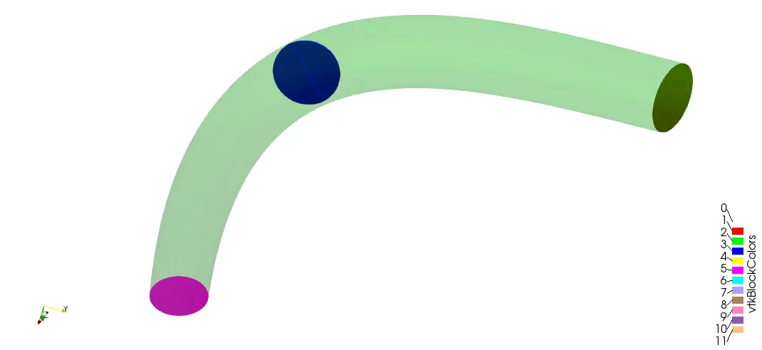
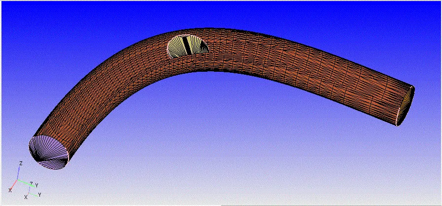
Image 1: Elbow body along with Throttle
*Each face of the step was split into multiple triangles.
The Geometry can be downloaded from this link: Elbow Geometry
To create the geometry, the geometry was uploaded from the different CAD software package. Then the geometry clean up was done along with inlet and outlet catch creation. All the normal vector were pointing out for this geometry, so we wanted it to point inside and normal to each surface. Normals point the direction of the fluid region generally. The command "Transform" was used to make the normal inside pointing the direction of the fluid region.
The Geometry was a check for if the geometry has any open surface.
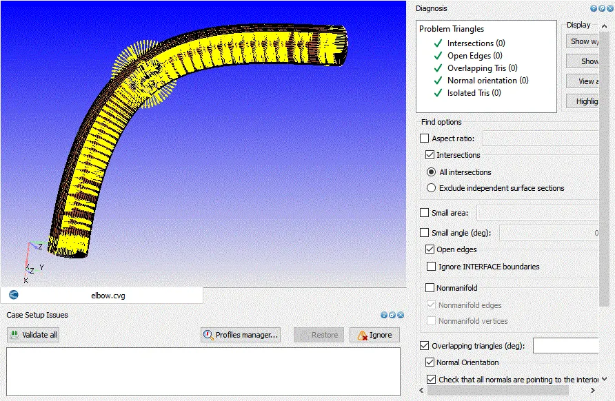
Then the normal ere checked and from the diagnostic dock, everything was checked.
2.Boundary Creation:
After creating the elbow Geometry, The Boundry tag was created along with different boundary id and coloring. A total of 4 different boundaries tag was created for so many different split triangles of the elbow with each face split into multiple triangles. To create the boundaries naming, the "Boundary" command in the "Geometry" dock was used, and then the faces were appointed to appropriate tags along with id.
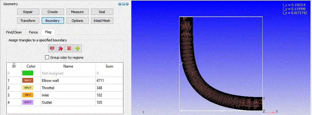
Image 2: Boundary creation representing the different id and color.
The five different boundaries were Inlet, Outlet, Elbow Wall, and Throttle.
3.Case-Study Setup:
The various parameter was considered while setup this case study. The case study setup dock was used to set up the problem which appears on the right-hand side of the converge studio.
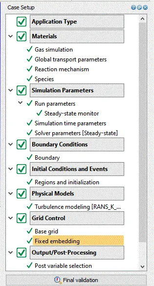
Image 3: Case Setup Dock.
3.1 Application Type:
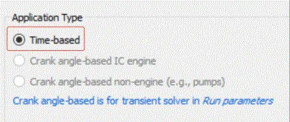
In order to run a steady-state simulation, firstly, under the Application type in the setup tree, a "Time-based" simulation must be selected.
3.2 Materials:
Under the material tab "Gas simulation" was selected and "Air" as a predefined mixture.
Gas: Air
Global Transport Parameters: Fixed value
by default, the following value is considered.
Prandtl Number : 0.9
Schmidt Number : 0.78
Species: Oxygen-O2 & Nitrogen-N2
Reaction Mechanism (mech.dat) was selected for this problem.
3.3 Simulation Parameters:
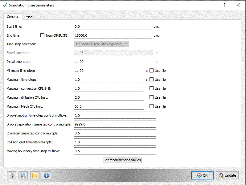
The Steady-state solver was selected for running this case study along with a "Pressure based" solver.
STEADY STATE SIMULATION:
These are the simulation we run if are just interested in the end result and not in how those results are getting formed with time. The time is in CYCLES for STEADY STATE SIMULATION.
The Following Simulation parameters were selected for running each simulation.
3.4: Boundary Conditions:
In this tab, The volumetric region and physics for each boundary were defined.
| Boundary_Name | Boundary_Type | Paramter_Defined | Boundary ID |
| 1.Inlet | Inflow | 150000.0 Pa | 3 |
| 2.Outlet | OutFlow | 100000.0 Pa | 4 |
| 3.Elbow Wall | Wall |
Specified Value(300k) Law of wall |
1 |
| 4.Throttle | Wall |
Specified Value(300k) Law of wall |
2 |
3.5: Initial Conditions and Events:
Volumetric Region was created in order to assign this to all the boundary tag.
Species:- O2 (0.23) & N2 (0.77)
Pressure :101325Pa
Temperature:300K
3.6: Physical Models
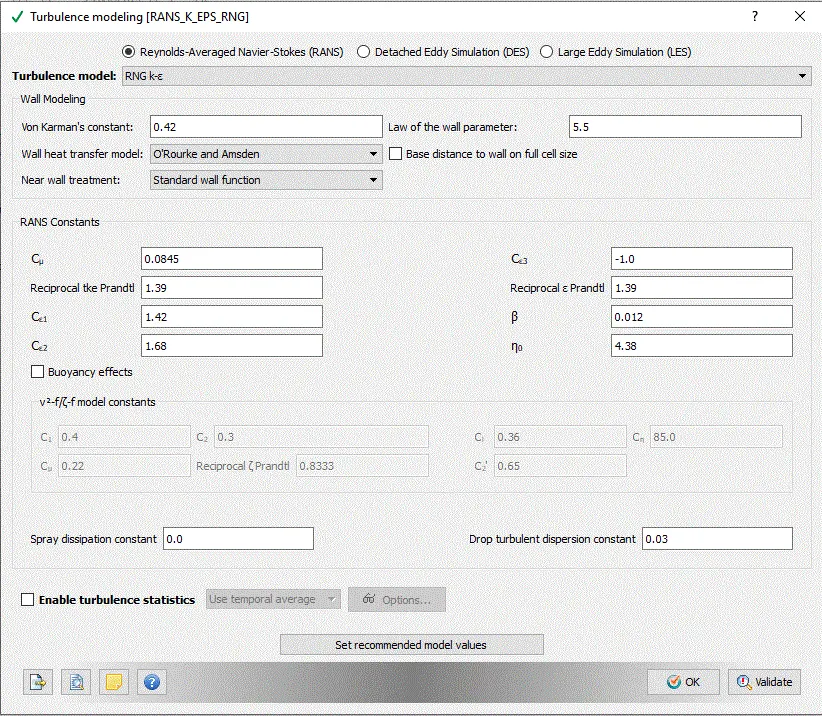
A turbulent model was selected out of so many models.
3.7: Grid Control:
The case study was run using fine different mesh grid size. So different case study was set up in order to study the effect of value when the mesh is more refined.
3 different base mesh sizes are,
| S.No. | Dx(m) | Dy(m) | Dz(m) |
| 1 | 0.004 | 0.004 | 0.004 |
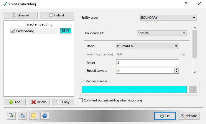
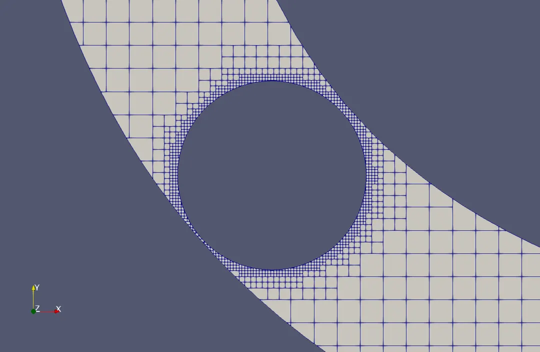
Fixed embedding was done in order to capture more cells near to throttle in order to get more precise data.
Scale : 3 & Embed Layers: 2
3.7: Output/Post-Processing:
Post-Variable Selection- Existing value
Output Files- Time interval for writing 3D output files-100.0
The time interval for writing restart files -1000.0
The case study was solved using CYGWIN and the post-processing was done in ParaView.
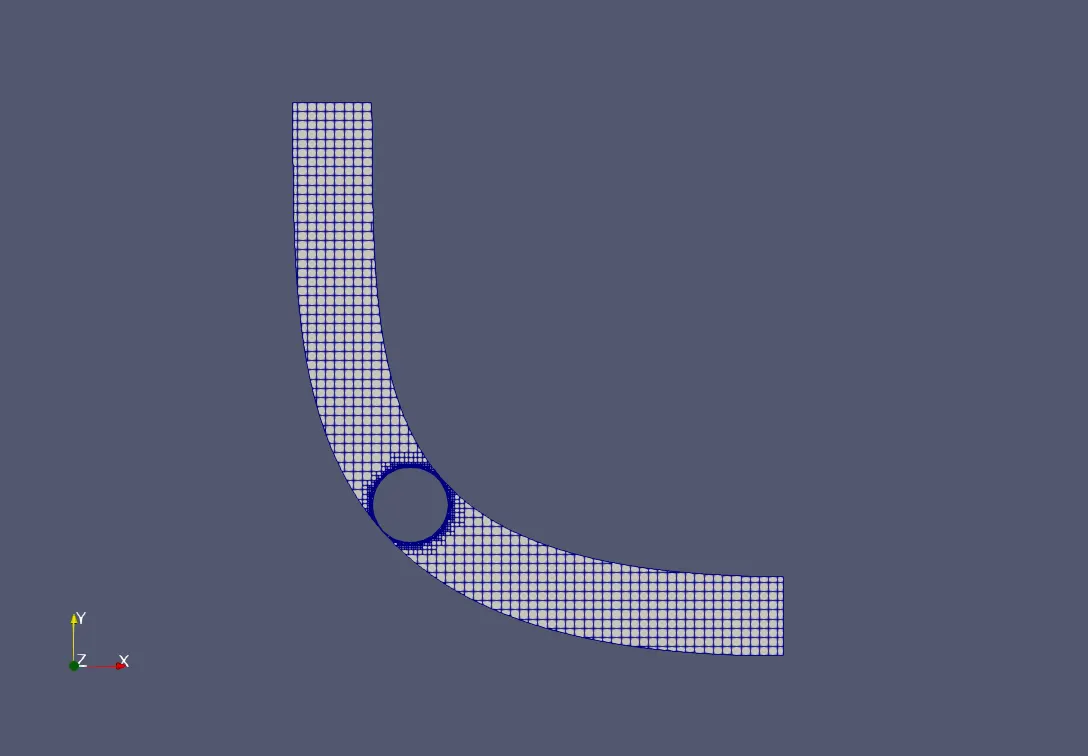
Meshed Geometry:
Case Study: dx=dy=dz=4e-3 m
Meshed Geometry with Fixed Embedding on Throttle.
Result: (Line Plots & Contours):
1)Velocity contour and Plot:
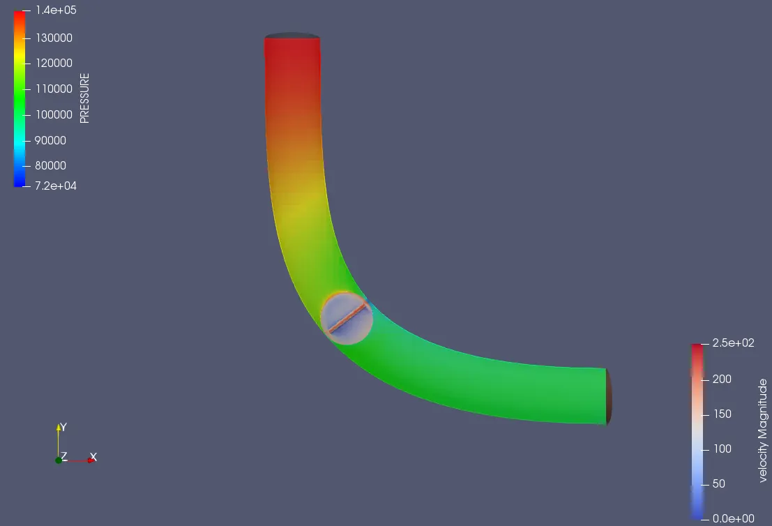
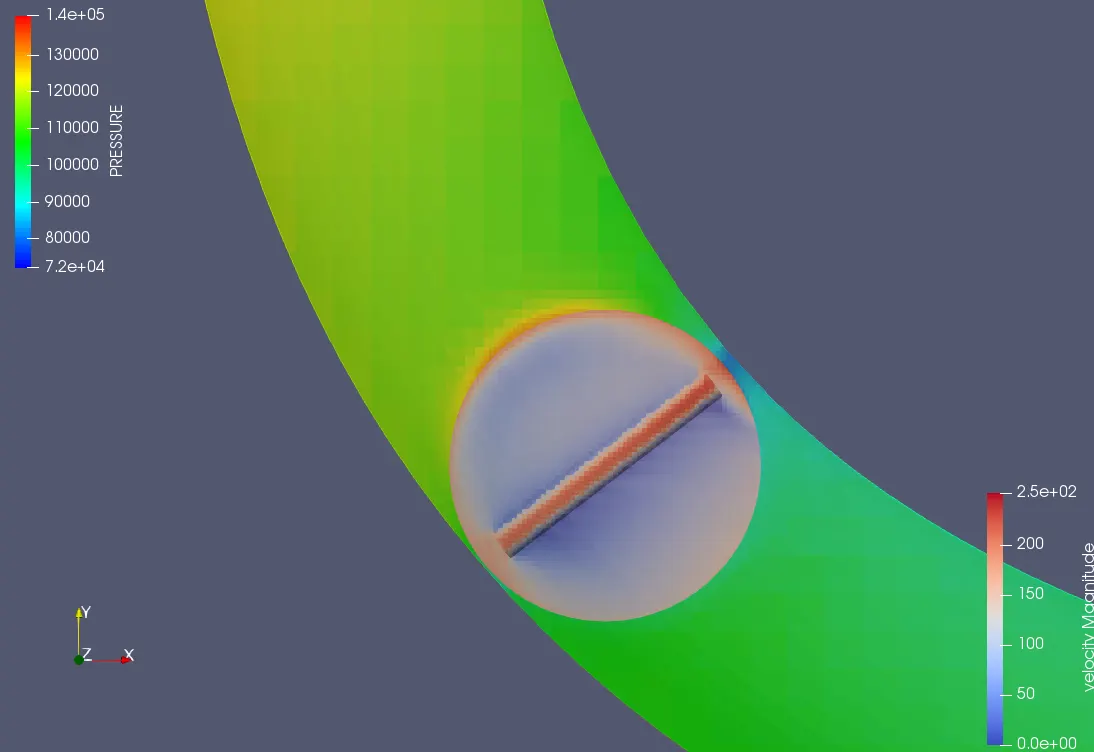
The velocity contour of a section cut along the plane normal to he z-axis is as shown below. The maximum velocity of 240m/s is predicted near the gapping between the throttle and elbow wall which is understandable due to the reduced flow area at that section and also lowest velocity is noticed behind the valve where is flow is obstructed.
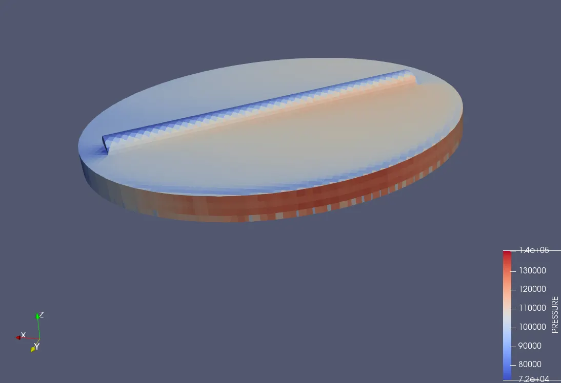
2)Pressure Contour and plot:
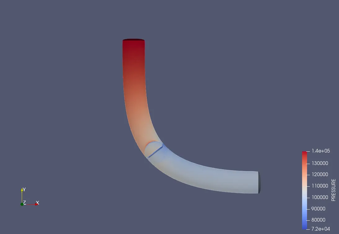
The Pressure contour of a section cut along the plane normal to he z-axis is as shown below. The maximum pressure of 1.4 Bar is predicted near the gapping between the throttle and elbow wall which is understandable due to the reduced flow area at that section and also the pressure of .5 bar is noticed behind the valve where is flow is obstructed.
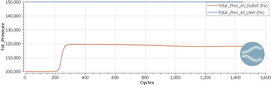
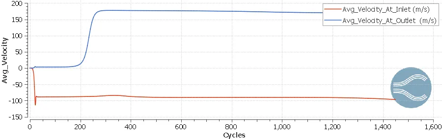
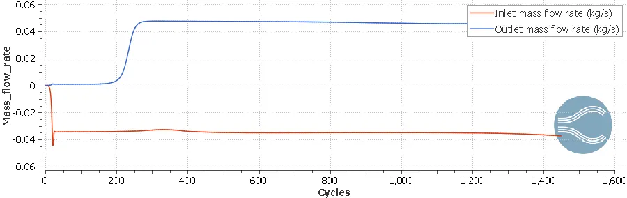
3)Average Mass flow:
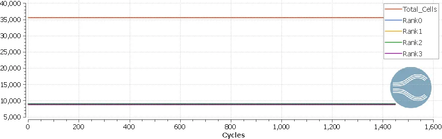
4)Total Cells:
The Youtube link for the animation of velocity and pressure contours are given below,
Conclusion:
- Graph for the average mass flow rate through both inlet and outlet for thus case- The mass flow rate after 1200 cycles approx.
- The outflow and inflow mass rate is equal to 0.05 kg/s approximately.
- The maximum pressure of 1.4 Bar is predicted near the gapping between the throttle and elbow wall which is understandable due to the reduced flow area at that section and also the pressure of 0.5 bar is noticed behind the valve where is flow is obstructed.
- The maximum velocity of 240m/s is predicted near the gapping between the throttle and elbow wall which is understandable due to the reduced flow area at that section and also lowest velocity is noticed behind the valve where is flow is obstructed.
- The total number of cells was found to be nearly 36,000. The Fixed Embedding option helped to capture more number of the cell near to elbow wall and throttle.
The Case Study can be downloaded from here: