Rayleigh Taylor Instability Challenge

Rayleigh-Taylor Instability Analysis

Two fluids of different densities superposed over each other (or accelerated towards each other); the instability of the plane interface between the two fluids, when it occurs, is called the Rayleigh-Taylor instability.

In the context of the Rayleigh-Taylor instability, there are two fluids being considered, one above the other, which are separated by a horizontal plane.

If the lighter fluid is above the heavy fluid, the interface between the two is “stable” because the heavy stuff may be considered to have already fallen and the light stuff has already risen. Stable does not imply there is no motion, if there is air above a water surface, a 2 displacement of the surface will result in waves traveling horizontally on the surface.

PART A:

Some practical CFD models that have been based on the mathematical analysis of Rayleigh Taylor instability are-

The Kelvin–Helmholtz instability

The Kelvin–Helmholtz instability can occur when there is velocity shear in a single continuous fluid or where there is a velocity difference across the interface between two fluids. An example is a wind blowing over water.

The Plateau–Rayleigh instability

The Plateau–Rayleigh instability, often just called the Rayleigh instability, explains why and how a falling stream of fluid breaks up into smaller packets with the same volume but less surface area. It is related to the Rayleigh-Taylor Instability and is part of a greater branch of fluid dynamics concerned with fluid thread breakup.

Richtmyer–Meshkov instability (RMI)

The Richtmyer–Meshkov instability (RMI) occurs when two fluids of different density are impulsively accelerated. Normally this is by the passage of a shove wave. The development of the instability begins with small amplitude perturbations which initially grow linearly with time. This instability can be considered the impulsive-acceleration limit of the Rayleigh-Taylor Instability.

PART B:

Rayleigh Taylor instability simulation for 3 different mesh sizes with base mesh (0.5 mm). Lighter fluid in the first 3 cases is the air on the bottom and heavy fluid is water on top.

Case 1- Base Mesh (0.5mm)

Mesh

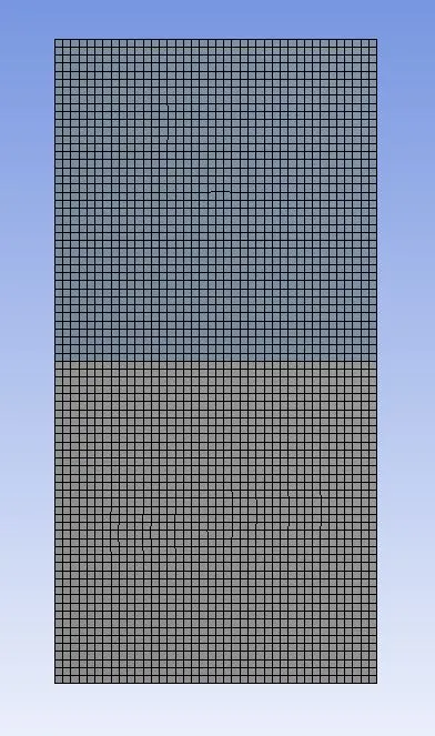
Statistics of mesh:

Number of Nodes - 3321

Number of Elements - 3200

Video of Simulation

Case 2- 0.3mm

Mesh

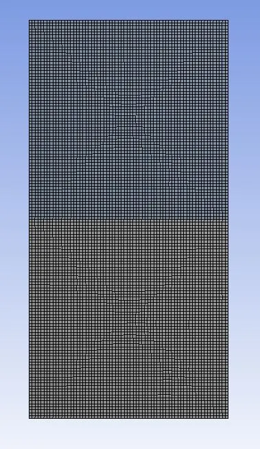
Statistics of mesh:

Number of Nodes - 9180

Number of Elements - 8978

Video of Simulation

Case 3- 0.2 mm

Mesh-

Statistics of mesh:

Number of Nodes - 20301

Number of Elements - 20000

Video of Simulation

Effect of mesh sizing

We can draw an observation from case 1 to case 2 to case 3, as element size reduces the bubble formation increases.

Why not a steady-state simulation?

Steady-state is not used in this case since in steady-state we get the behavior of fluid which is independent of time but in here we need to study instability at the interface from the instant when it starts which help to get a better idea how heavy density fluid get mixed and lighter density fluid rise above with respect to the time domain.

PART C:

Case 4- 0.2 mm

In this case unlike the above 3 cases instead of air, user-defined fluid is taken with properties as, density = 400 kg/m³, viscosity = 0.001 kg/m-s.

Rayleigh Taylor instability simulation with water and user-defined material. (for refined mesh)

Video of Simulation

The steady-state analysis in CFD always gives the end result of the fluid behavior.

In this simulation, we want to study the instability of the 2 different fluid from the moment it mixed together until the steady-state is reached, we need to capture the physical phenomena at each time step, therefore we used transient simulation which is time-dependent.

PART D:

Atwood Number

The Atwood number (A) is a dimensionless number in fluid dynamics used in the study of hydrodynamic instabilities in density stratified flows. It is a dimensionless density ratio defined as-

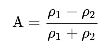
Where,

= density of a heavier fluid

= density of a lighter fluid

For case 1,case 2 and case 2:

heavier fluid(water)

density 1=998.2 kg/m^3

lighter fluid(air)

density 2=1.225 kg/m^3

Atwood number(A) =(density 1-density2)/(density 1+density2)

Atwood number(A)=0.996

for case 4:

heavier fluid(water)

density 1=998.2 kg/m^3

lighter fluid(user-defined material)

density 2=400 kg/m^3

Atwood number(A) =(density 1-density2)/(density 1+density2)

Atwood number(A)=0.427

For Atwood number close to 0, RT instability flows take the form of symmetric “fingers” of fluid;

For Atwood number close to 1, the much lighter fluid “below” the heavier fluid takes the form of larger bubble-like plumes.

Therefore, from the value of Atwood number, it is seen from the simulations that air forms larger bubbles when water is poured down the air pushes through and forms large bubbles. Therefore, the results can be validated by obtaining the value of the Atwood number.

Conclusion:

• For the case of small Atwood numbers, the difference in densities are small and the slow process of penetration are seen. RT instability flows take the form of symmetric fingers of fluid.
• With the increase in the Atwood number, there is a rapid process of penetration. Lighter fluid below the heavier fluid takes the form of larger bubble-like plumes and move against the gravity very fastly.
• With the Finer mesh, the instability captured properly and smaller bubbles are also visible in the finer mesh.