Exhaust Port Challenge
Exhaust Port Challenge
Title: To perform Conjugate Heat Transfer (CHT) Analysis with Exhaust Port Simulation.
- Introduction
Conjugate heat transfer (CHT) analysis is generally used when there is temperature variation during heating or cooling in the material due to the interaction between solid and fluid phases. It is the combination of heat transfer in solids to heat transfer in fluids.
Examples of Conjugate Heat transfer analysis:
HVAC, Heat Exchanger, Tank, Internal Combustion Engine, Heat Sink, Boiler, Reactor, Heat Pipe, Turbocharger.
The objective of this challenge is to perform a CHT analysis on the exhaust manifold model and to examine the velocity, temperature, and heat transfer coefficient at the outer wall.
- Solving & Modelling approach
To perform Conjugate Heat Transfer (CHT) Analysis with Exhaust Port Simulation with the help of ANSYS Fluent, proper setup of model geometry is needed with good quality meshing. To compare the results and value of the surface heat transfer coefficient on the internal solid surface, two cases are performed here with the different turbulence models namely k-epsilon and k-omega SST model.
2.1 Geometry
As we are interested in finding the surface heat transfer coefficient on the internal solid surface and the velocity distribution in a fluid in this simulation, we need to generate two volumes namely fluid-volume and solid-volume from these models using the volume extract feature from the SpaceClaim. Using the volume extract tool, we get a computational fluid domain as shown below.
Figures below show the solid-volume and fluid-volume that are being used for the simulation.
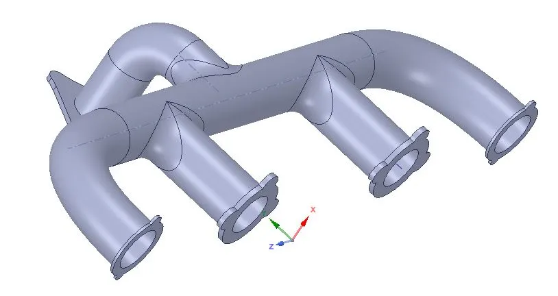
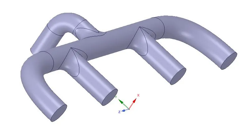
1) Solid volume 2) Fluid Volume
2.2 Meshing
After generating the computational fluid domain from the model, the next step is to discretize the fluid domain. ANSYS meshing tool is used to generate a mesh in the model.
2.2.1. Baseline mesh
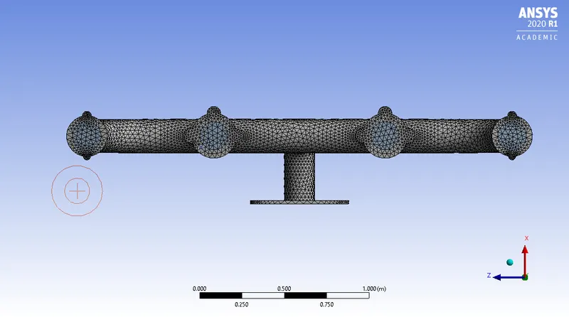
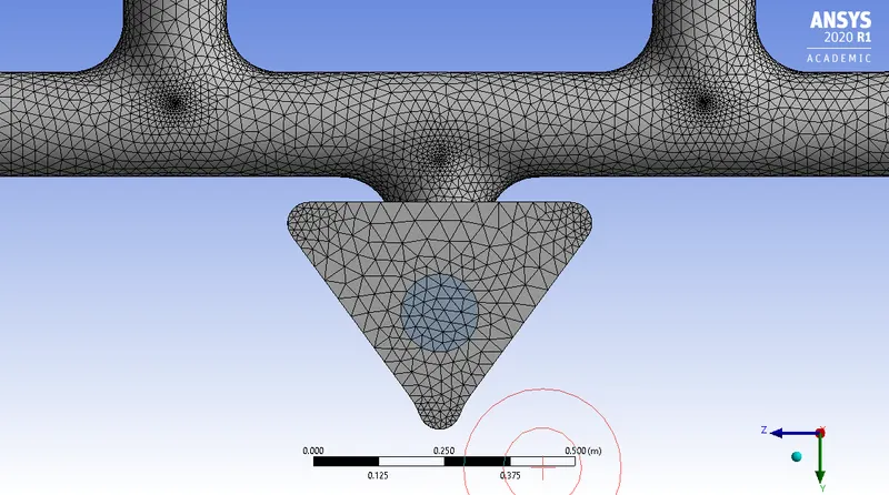
Statistic of mesh: Number of Nodes - 27381
Number of elements - 137286
2.2.2. Refined Mesh
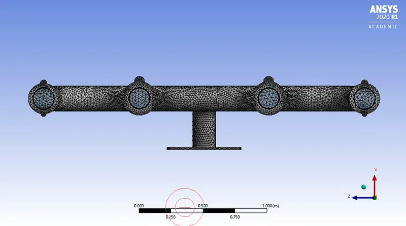
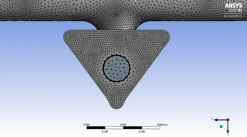
Statistic of mesh: Number of Nodes - 112954
Number of elements - 373840
2.2.3. Name selection in Model
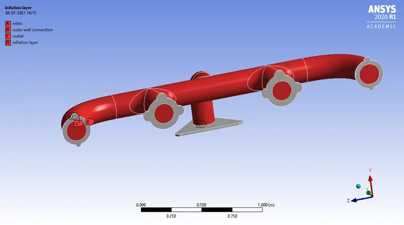
Figures above show the name selection for the final simulation setup.
- Pre-processing and solver setting
The next step in the simulation after generating fine meshing is to set-up the physical properties for the case.
The Energy equation needs to be enabled, as we are interested in solving for the Temperature distribution.
- Type of solver: Pressure-based
- Simulation method: Steady-state simulation
- Material of solid: Aluminium
- Material properties of fluid (Air)
Density: 1.225 kg/m3
Cp (Specific heat): 1006.43 J/kg-k
Thermal Conductivity: 0.0242 w/m-k
Viscosity: 1.7894e-05 kg/m-s
- Inlet velocity: 5 m/s
- Inlet Temperature: 700 K
- Outlet: Pressure type, 0 gauge pressure.
- Walls: wall type with no slip.
- Wall Heat Transfer Coefficient: 20 W/m²-k (Convection Heat Boundary)
- Turbulence Model: k-epsilon and k-omega SST model
- Results
4.1 Base Mesh result with the k-epsilon model.
Residual plot
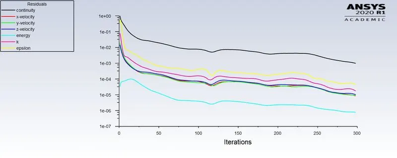
Velocity Streamline Profile
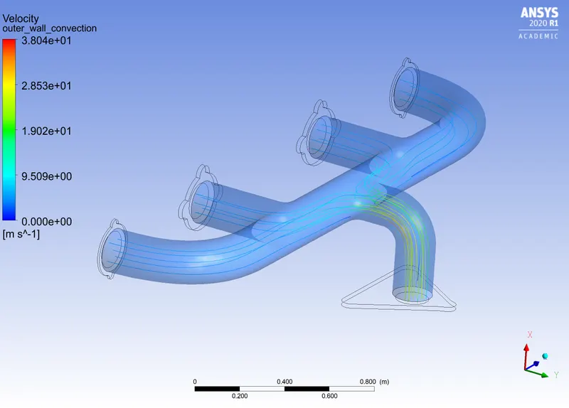
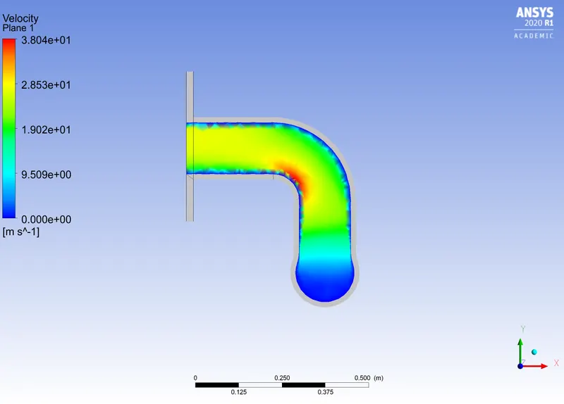
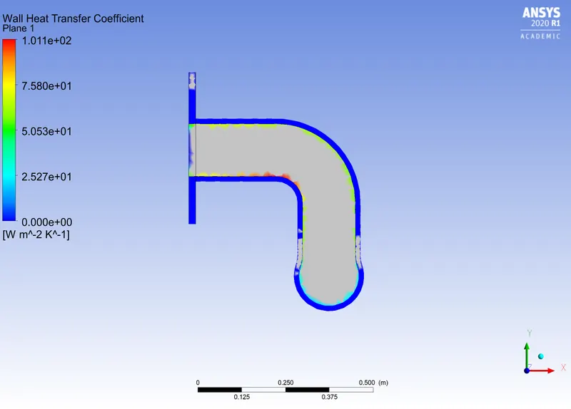
Velocity contour Wall Heat Transfer coefficient
4.2 Base Mesh result with the k-omega sst model.
Residual plot
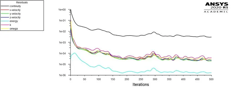
Velocity Streamline Profile
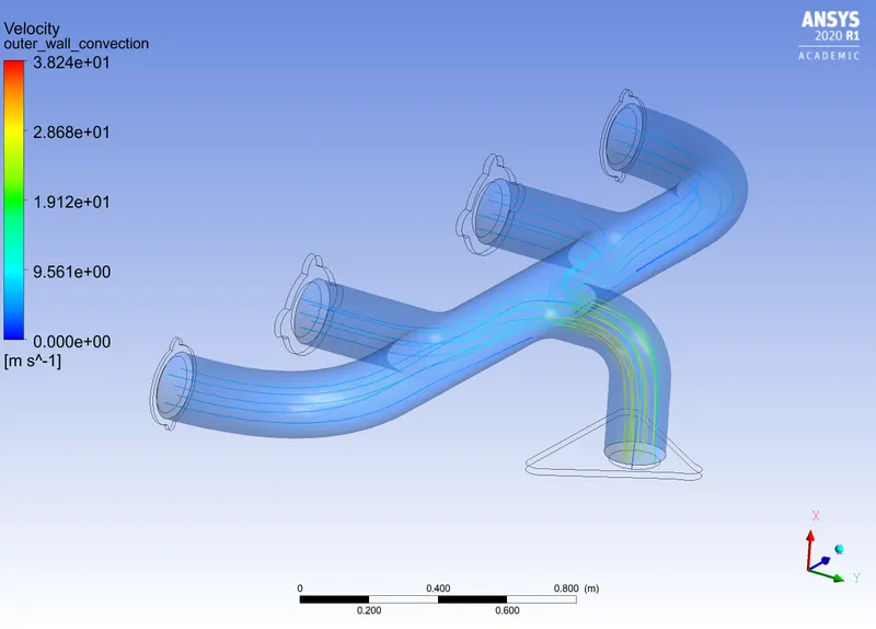
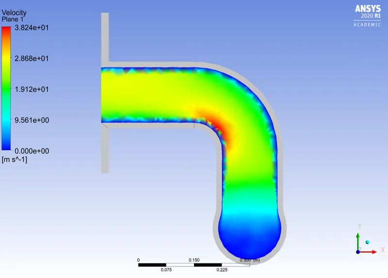
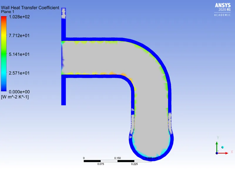
Velocity contour Wall Heat Transfer coefficient
4.3 Refined Mesh result with the k-epsilon model.
Residual plot
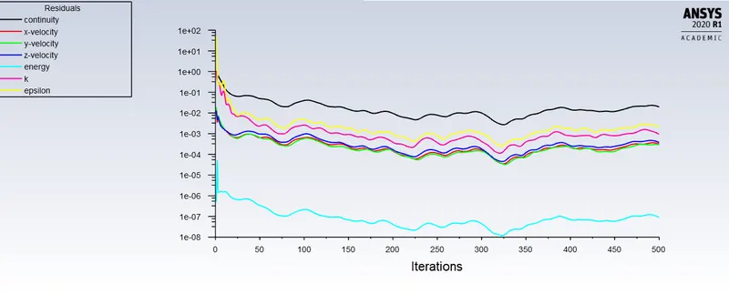
Velocity Streamline Profile
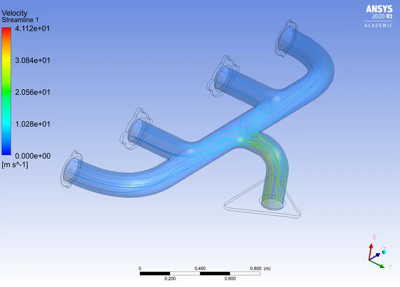
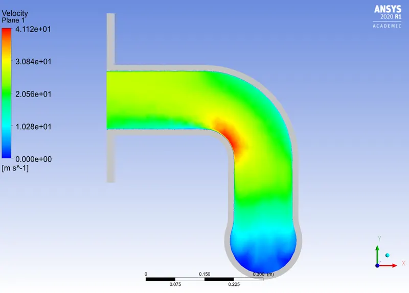
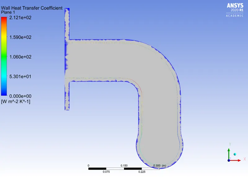
Velocity contour Wall Heat Transfer coefficient
4.4 Refined Mesh result with the k-omega sst model.
Residual plot
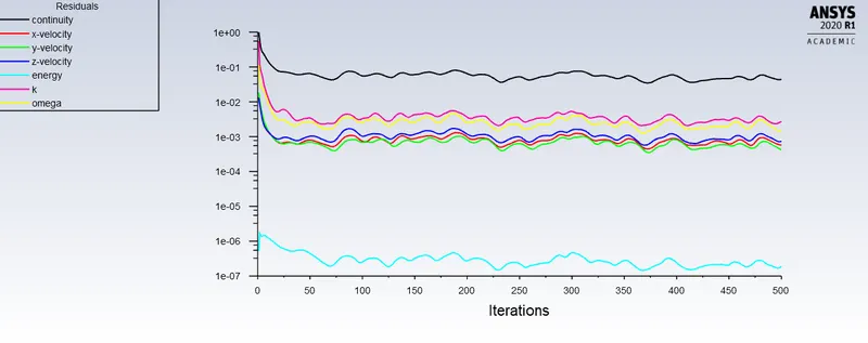
Velocity Streamline Profile
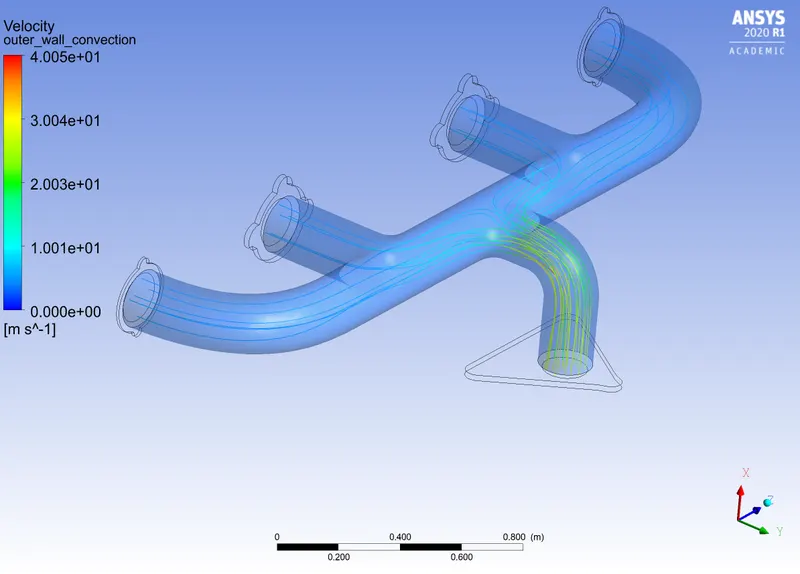
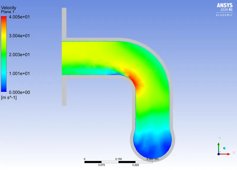
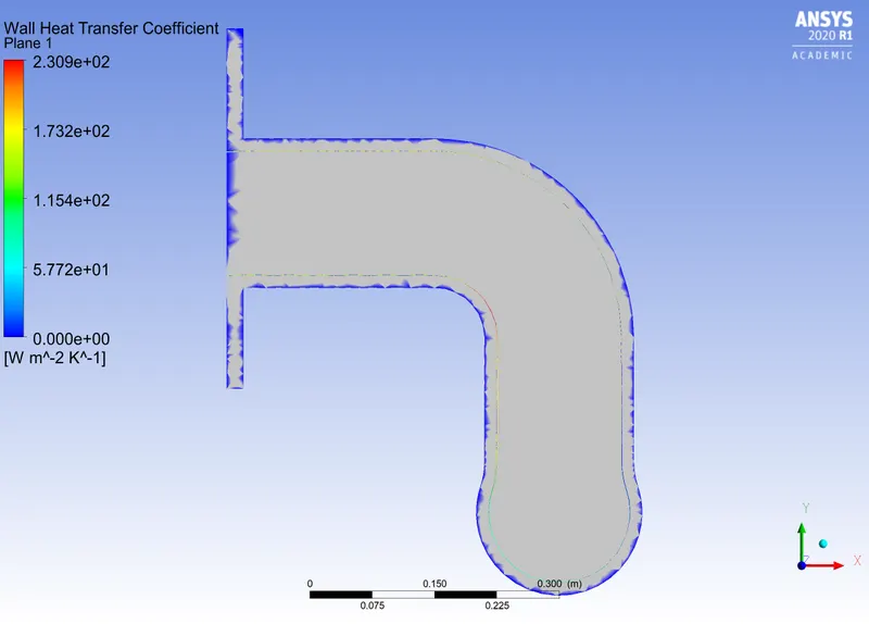
Velocity contour Wall Heat Transfer coefficient
The validity of Simulation results
1. The accuracy of the simulation results is validated by comparing it with the available experimental data from reserach paper.
2. The accuarcy of the result can also be validated by performing grid dependency test.
3. The validation of the simulation results can be numerically verfied by theoretically calculating Nusselt number to find heat transfer coefficient.
Nusselt Number:
It is a dimensionless parameter used in calculations of heat transfer between a moving fluid and a solid body. It is the ratio of heat transferred through convection (fluid motion) to the heat transferred through conduction. This number gives the quantification of the heat transfer occured due to fluid motion.

here,
D = Diameter of the circular duct,
Pr = Prandtl number,
n = 0.4 for the fluid being heated, and n = 0.3 for the fluid being cooled.
Nu = Nusselt Number
Re = Renolds number
By examining the velocity contours at the plane we can understand that there is the high velocity at the bent which implies high Reynold number. From the above relation, we can say that as Re increases Nu increases as well, which in turn increases the heat transfer coefficient.
Factors affecting the accuracy of the simulation results
1. The quality of mesh - Finer and well defiened mesh gives more accurate results.
2. Inflation layers around the critical surface for the flow.
3. Accurate fitting of mesh around the geometry - Mesh needs to accurately accommodate the geometry around the curvatures
4. Setting share topology - Mesh should be conformal for smooth transferring of mesh in different zones.
- Conclusion
1. The results are more accurate in the second case as compared with the first case due to the mesh refinement.
2. There is no change in temperature difference in both cases but the change in minimum temperature, it is in the second case because of mesh refinement.
3. The wall coefficient heat transfer also increases in the second case.
4. The velocity and hence the Reynolds number, is higher at the outlet. Due to that, the heat transfer and temperature is higher.
5. The heat transfer coefficient is higher between fluid and solid at outlet pipe, because the velocity of the fluid is higher.