FSAE Car Project
FSAE Car Project:
Aim:
The major objective of this project was to Setup Aerodynamics Simulation of a Formula Student Type race car using Converge CFD and Estimate the Drag and Lift force on different major components.
Introduction:
The project's aim is to Study the external fluid dynamics of racing cars. The study of aerodynamics provides an interesting application for illustrating principles of fluid mechanics. Race cars are aerodynamically designed to reduce drag force or decrease vehicle’s resistance and enhance downforce. Drag forces limit maximum speed and affect fuel consumption although downforce is used to provide stability when driving around corners. The CFD is very useful in the automobile industry from the system level to the component level to analyze the fluid flows. In the present paper, the effect of aerodynamics on various parameters of a racing car and CFD has been reviewed briefly.
The report contains a detailed description of two different case studies:-
Race-1
- Racing track conditions - Straights
- Average lap speed - 75kmph
Race-2
Racing track conditions - Lot of turns
- Average lap speeds - 45kmph
- 70% turns at 45 degrees
- 20% turns at 80 degrees
- 10% turns at 20 degrees
The project mainly focuses on the following things:-
1. Importing the(.Stl) file on Converge Studio then cleaning up the geometry removing the intersection, patching the new open edge, deleting the unwanted edge, and Fixing the normal orientation of the geometry.
2. Creating Virtual Wind Tunnel using proper Dimension.
3. Case Setup using Converge Studio using proper Solver and Boundary Conditions.
4. Solving the Case Study Files using Cygwin.
5. Post-Processing the result Using ParaView generating Velocity, Pressure, and y+ contours.
6. Generating the plots and comparing the result for Drag and Lift force using Ms. Excell.
--------------------------------------------------------------------------------
1. Importing the Geometry for Geometry Clean Up using Converge Studio
Firstly the Geometry(.stl) was imported in Converge Studio. The diagnostic tool was used to find the open edge, Intersection edges, and other errors like orientation error. Many features were used to repair the geometry like 1. Deleting the edge, node, face. 2. Patching the edge using the patch tool. 3. Stitching the two misalign edges.
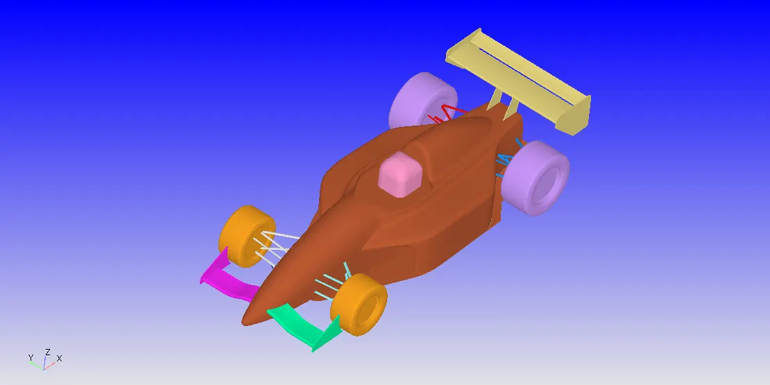
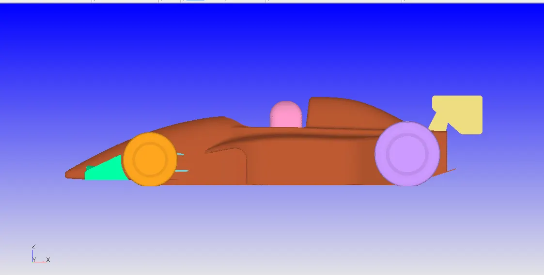
The car geometry that was provided had 48 total open edge errors. so geometry cleaning plays an important role in setting up a simulation of a car. There were many features that were used to clean the geometry. First, the geometry was checked using the Diagnostic tool to check what kind of error is present then our main target was to repair an open edge without forming an intersection.
First, the surface(Triangle) was deleted shown in green color then the extra edges were removed to make a perfect open loop that can be patch letter. For patching those new open edge the edges were checked and patch repair option was used to patch the open edge method. Then the geometry was checked again to find any error.
The normal orientation was fixed using automatic option present in Transform>Normal> Automatic fix all the normals.
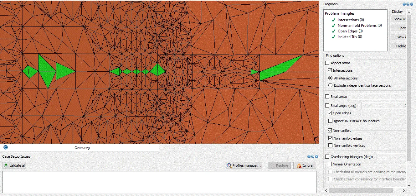
After doing Geometry clean up, The geometry was again finally checked for any error using the Diagnostic tool. At last, all the 48 errors were repaired as shown in the above picture.
Case Study Set-Up
1.Geometry Creation
First of all, the FSAE car geometry was imported using converge CFD software. The geometry was separately prepared using different CAD package ie Solidworks, then .stl file was imported to Converge Studio to set up the case study. Then the geometry clean up was performed in order to check for errors.
The Geometry was scaled using proper scale because the geometry was prepared using Inch so for that the geometry was converted in Metre using Scale feature.
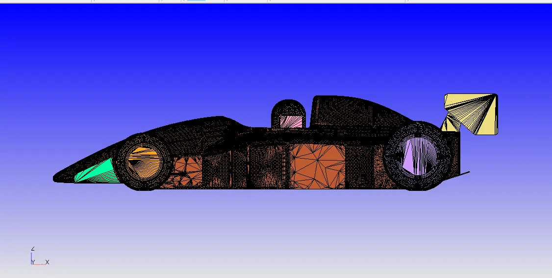
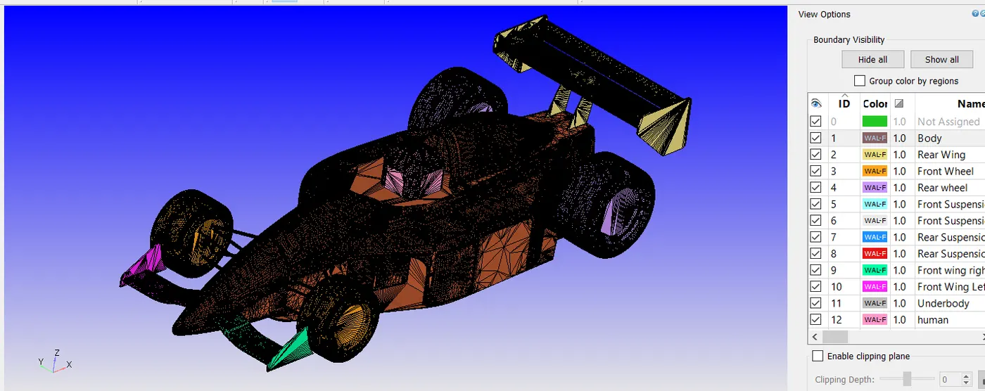
After the geometry was cleaned than the Virtual wind tunnel was created.
The Distance behind the FSAE car around 10 times the wheelbase of Car.
The Distance Infront of the FSAE car was taken around 4 times the wheelbase of the Car.
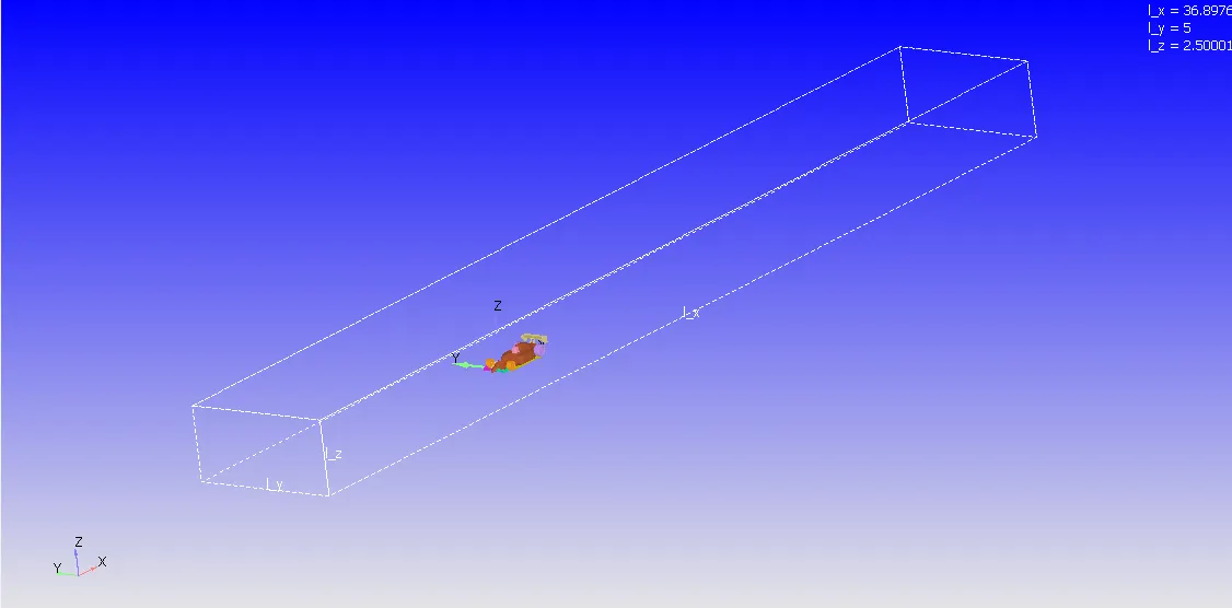
For Case1 The car was kept Straight
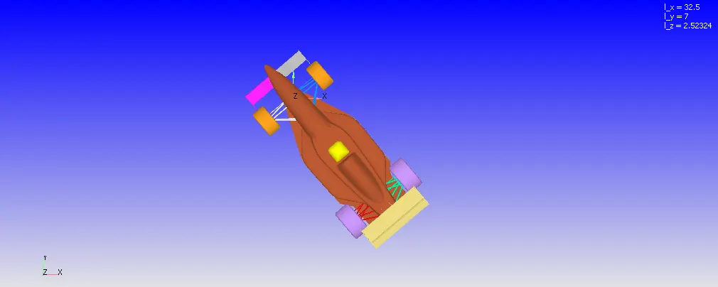
For Case2 The condition was during turning
Racing track conditions - Lot of turns
- Average lap speeds - 45kmph
- 70% turns at 45 degrees
- 20% turns at 80 degrees
- 10% turns at 20 degrees
The car Model was rotated along Z-Axis
`"Weight Average"=((0.70X45)+(0.20X80)+(0.10X20))/(0.70+0.80+0.20)=49.5Deg`
The Virtual Wind Tunnel Dimension for Case 1 is :
| Dx(m) | Dy(m) | Dz(m) |
| 36.8 | 5 | 2.5 |
The Virtual Wind Tunnel Dimension for Case 2 is :
| Dx(m) | Dy(m) | Dz(m) |
| 32.5 | 7 | 2.52 |
To create the geometry, the geometry was uploaded from the different CAD software package. All the normal vector were pointing out for this geometry, so we wanted it to point inside and normal to each surface. Normals point the direction of the fluid region generally. The command "Transform" was used to make the normal inside pointing the direction of the fluid region.
2.Boundary Creation
After creating the Geometry along with Wind Tunnel Geometry, The Boundry tag was created along with different boundary id and coloring. A total of 16 different boundaries tag was created for multiple different split triangles of the geometry with each face split into multiple triangles. To create the boundaries naming, the "Boundary" command in the "Geometry" dock was used, and then the faces were appointed to appropriate tags along with id.
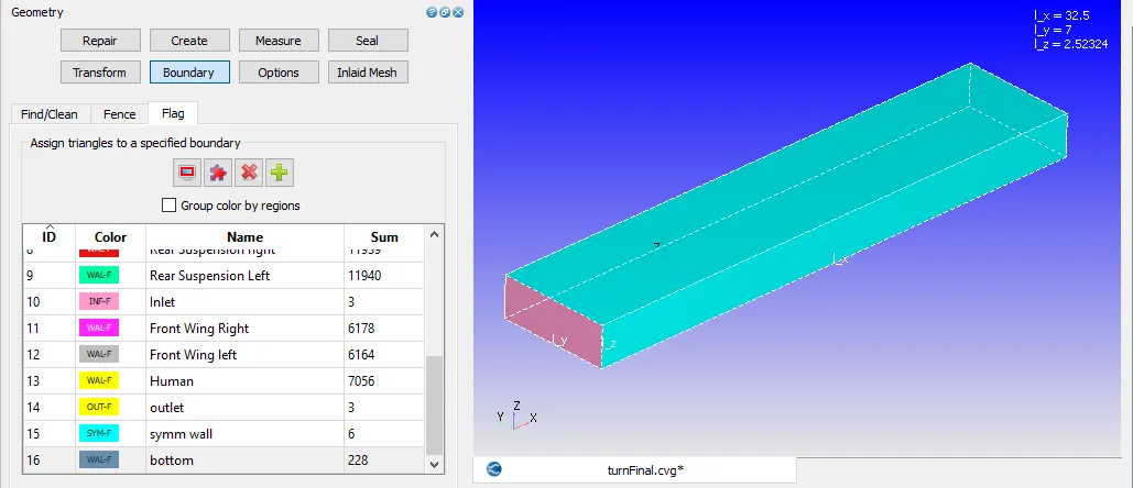
First, the FSAE car Geometry was split into many parts using Boundary Fencing Method using those parts the Boundary tag was created.
Then the Inlet, Outlet, Symmetry walls, and Bottom walls were created.
3.Case-Study Setup
The various parameter was considered while setup this case study. The case study setup dock was used to set up the problem which appears on the right-hand side of the converge studio.
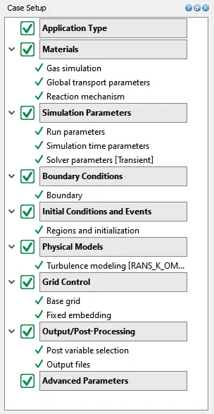
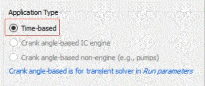
3.1 Application Type:
In order to run a steady-state simulation, firstly, under the Application type in the setup tree, a "Time-based" simulation must be selected.
3.2 Materials:
Under the material tab "Gas simulation" was selected and "Air" as a predefined mixture.
Gas: Air
Global Transport Parameters: Fixed value
by default, the following value is considered.
Prandtl Number : 0.9
Schmidt Number : 0.78
Species: Oxygen-O2 & Nitrogen-N2
3.3 Simulation Parameters
The Transient solver was selected for running this case study along with a "Density-based" solver.
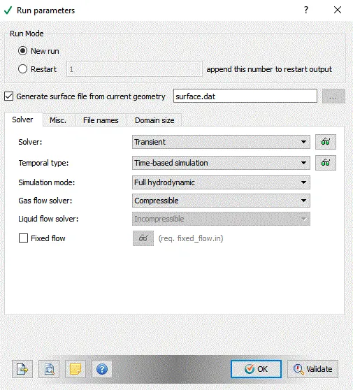
Calculation
Horizontal length=32.5m
Average Velocity for Case 1=12.5m/s
Average Velocity for Case 2=20.83m/s
Speed=Distance/time
therefore, Time=2.6 sec
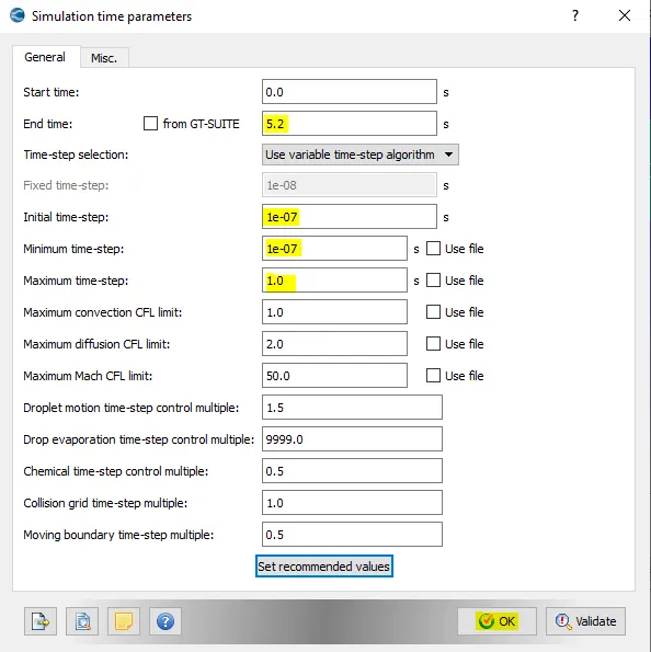
we are simulating roughly 2 times of flow through time that is 5.6s
The Following Simulation parameters were selected for running this simulation.
3.4: Boundary Conditions
In this tab, The volumetric region and physics for each boundary were defined.
| Boundary_Name | Boundary_Type | Paramter_Defined | Boundary ID |
| 1. Body | Wall | Law of Wall | 1 |
| 2. Rear Wings | Wall | law of Wall | 2 |
| 3. Front Wheels | Wall | law of Wall | 3 |
| 4. Rear Wheel | Wall |
law of Wall |
4 |
| 5. Undertray | Wall | law of Wall | 5 |
| 6. Front Suspension Right | Wall |
law of Wall |
6 |
| 7. Front Suspension Left | Wall |
law of Wall |
7 |
| 8. Rear Suspension Right | Wall |
law of Wall |
8 |
| 9. Rear Suspension Left | Wall |
law of Wall |
9 |
| 10. Inlet | Inflow |
12.5m/s in X-axis Case1 20.8m/s in X-axis Case2 (Dirichlet Boundary Condition) The pressure being at NE (Neuman Boundary condition) |
10 |
| 11. Front Wing Right | Wall | law of Wall | 11 |
| 12. Front Wing Left | Wall | law of Wall | 12 |
| 13. Human | Wall | law of Wall | 13 |
| 14. Outlet | Outflow |
101325.0 Pa at 300 k (Dirichlet Boundary Condition) |
14 |
| 15. Symm Wall | Symmetry | law of Wall | 15 |
| 16. Bottom | Wall | law of Wall | 16 |
3.5: Initial Conditions and Events
Volumetric Region was created in order to assign this to all the boundary tag.
Species:- O2 (0.23) & N2 (0.77)
Pressure :101325Pa
Temperature:300K
The velocity of 40m/s in X-axis
3.6: Physical Models
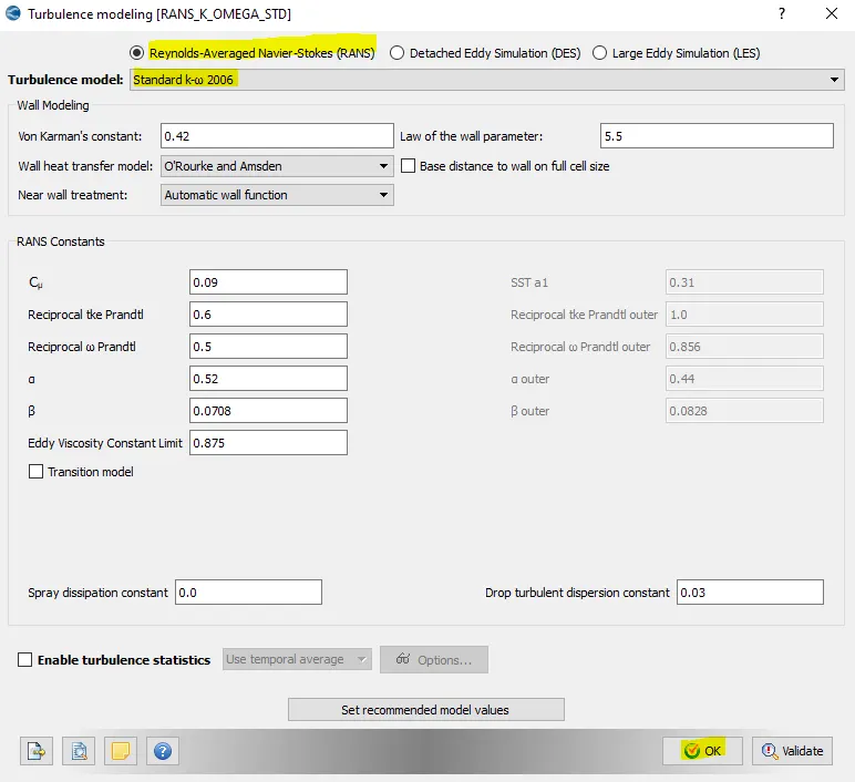
A turbulent model was selected out of so many models. RANS standard K-omega SST model was chosen.
3.7: Grid Control
The case study was run using a Coarse mesh grid size due to less computational resources.
Base mesh sizes are,
| S.No. | Dx(m) | Dy(m) | Dz(m) |
| 1 | 0.5 | 0.5 | 0.5 |
Fixed Embedding
Fixed embedding was done in order to capture more cells near to throttle in order to get more precise data.
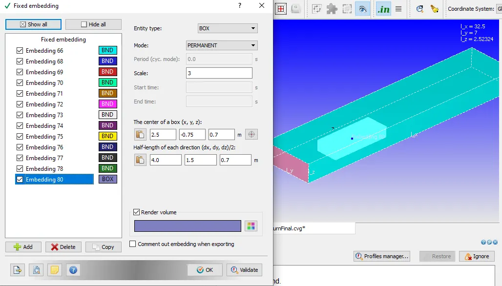
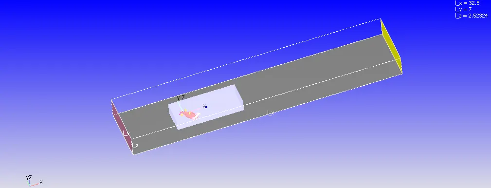
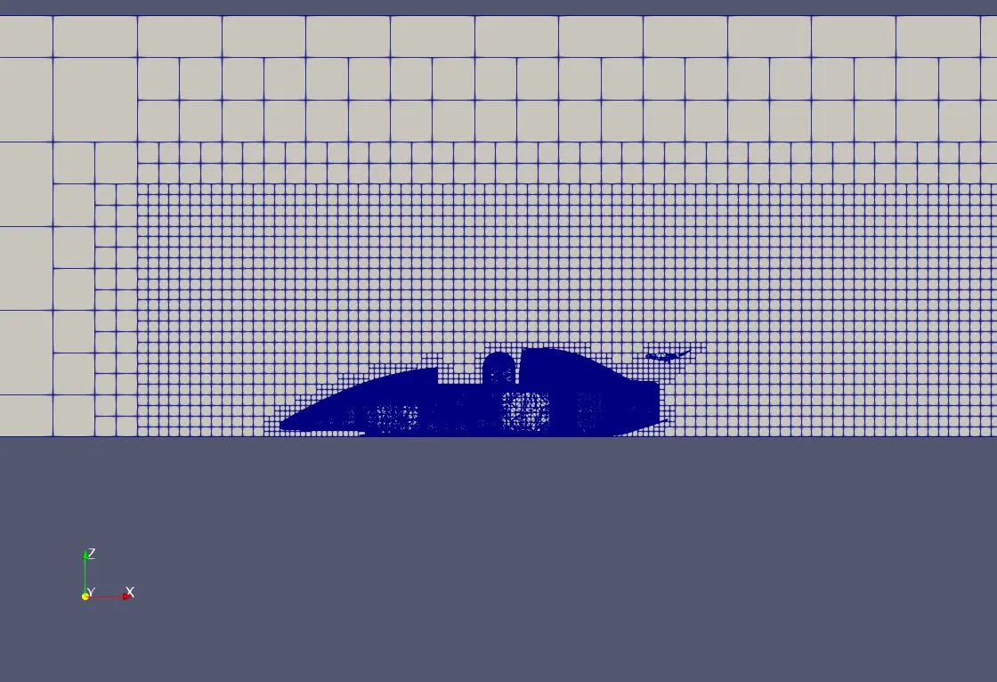
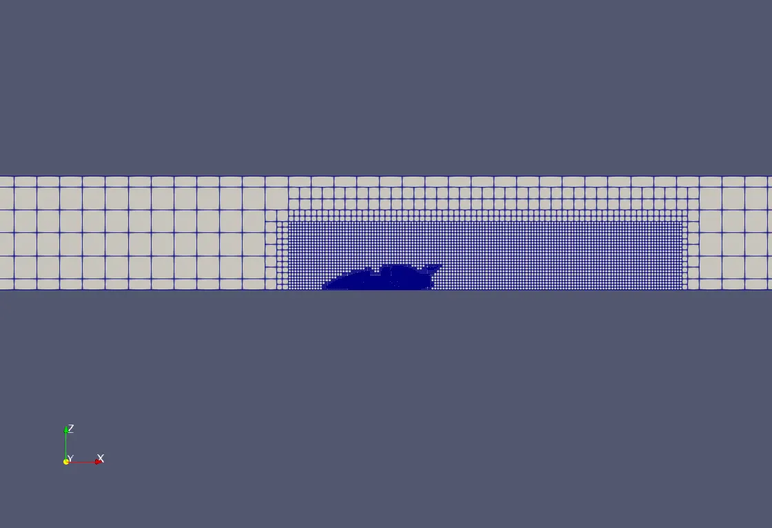
Wind tunnel that has box embedded inside with more fine computational cells in order to capture more data more precisely.
3.7 Output/Post-Processing
In regions and initialization, the value of velocity should be the same as that of Inlet velocity.
Also, while setting up the case, make sure, wall output (BOUNDARIES ONLY) is enabled as this will dump wall averaged output data which is very much important for any external aerodynamic simulations.
Post-Variable Selection- Existing value
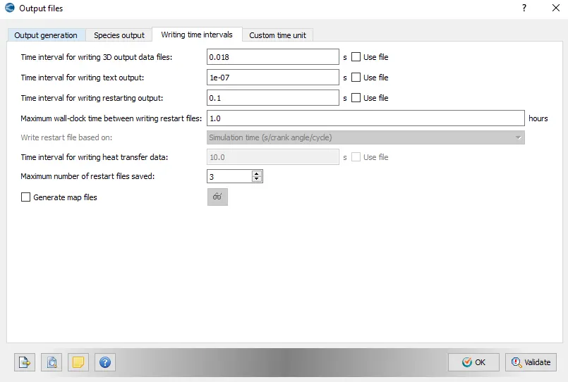
Output Files- Time interval for writing 3D output files-0.018 s
The time interval for writing restart files -0.1s
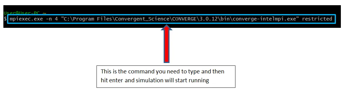
The case study was solved using CYGWIN and the post-processing was done in ParaView.
Simulation Results
Mesh Model
Case 1
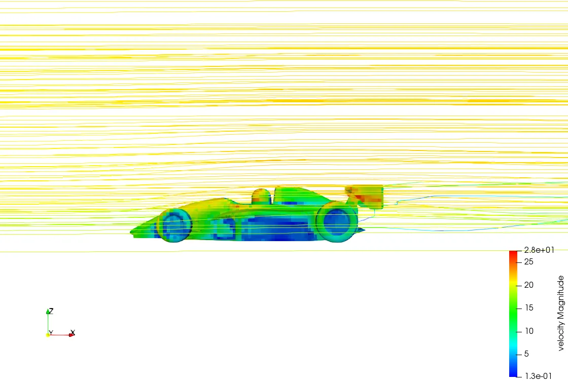
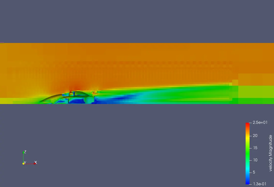
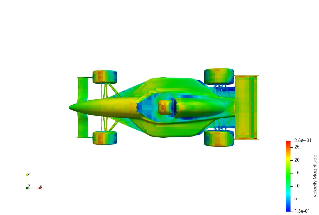
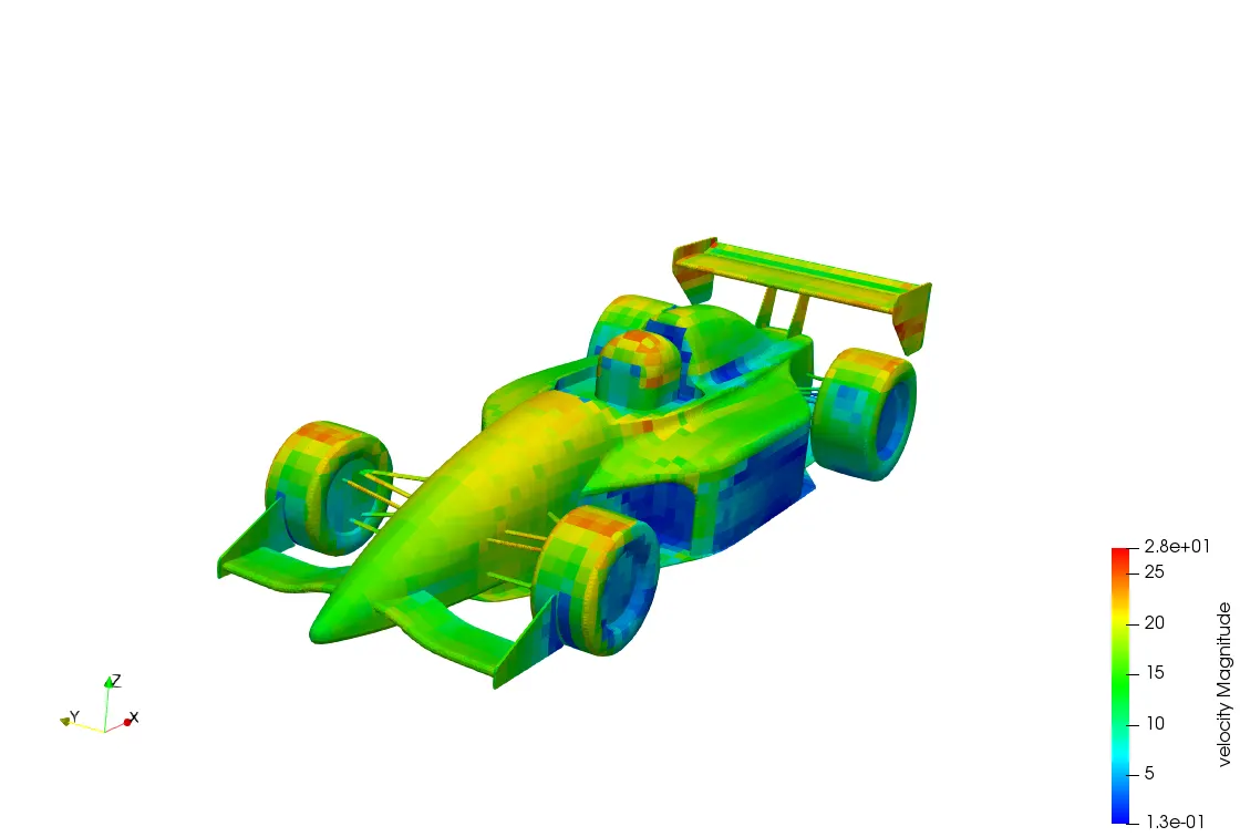
Velocity Contour
Observation
The velocity is much higher found above the car indicated in red color whereas very low in the down region and the side region of the car indicated with blue color. The velocity is less to an extent in front os the car that is the windward side. The main thing that can be noticed that the velocity is changing due to the aerodynamic device used in the car that is undertray that is providing the downforce and wing that has high-velocity fluctuation due to change in pressure.
Interference
As the air that is the working fluid, in this case, strikes the car, it loses its kinetic energy which leads to a decrease in the velocity of the fluid in the windward side of the car.
the fluid that strikes on the car is diverted to the upper part of it, which adds up to the velocity of the fluid actually flowing above the car, thus an increase in velocity is noticed above the car due to the nice aerodynamics design of the car.
Some amount of flow is diverted to the side of the car it is due to the front wings of the car and front wings can be designed in such a way to generate the vortex so that it does not interrupt the wheel while the car is on the race track so as to reduce the tire drag.
There is a flow separation that can be seen behind the car near to rear wings it is due to change in air pressure on the NACA aerofoil that is being used in. Wings and there is also a drop in velocity that can be seen behind the car because of drop-in pressure. Due to flow separation a region of partial vacuum is formed in the leeward side of the car this leads to recirculation of air and this gives rise to vortex formation. These Vortexes tend to move along the wind direction and this entire region of low velocity in along the leeward side of the car is also called at Wake region.
Pressure Contour
Observation
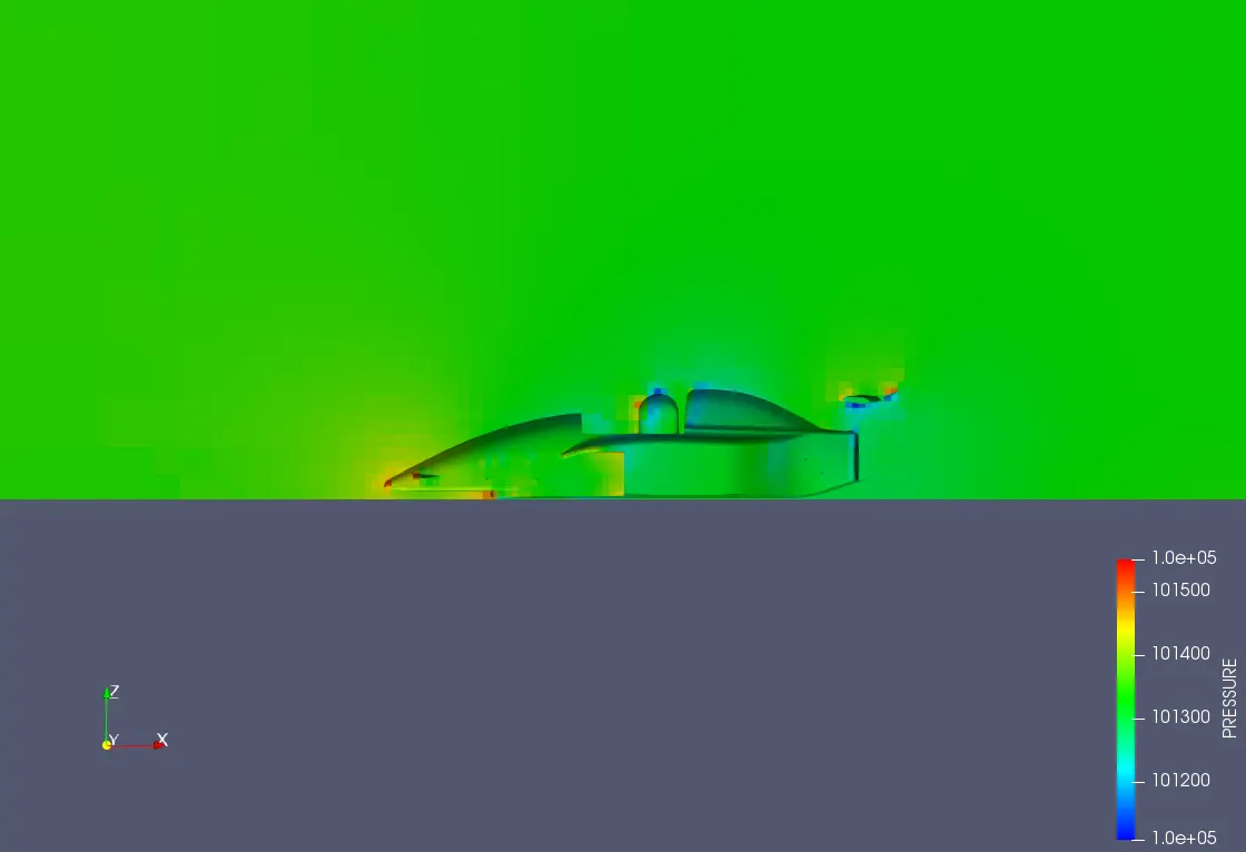
The pressure is much high on the region where airstrikes directly that is the front wings wheel body, human, etc. indicated in the red region.
The pressure is relatively lower in the upper and leeward side of the car indicated with blue color.
Interference:
As the airstrikes, the car, the kinetic energy of the car is converted into pressure energy thus the increase in pressure in the front part of the car which incident to the free stream that is responsible for drag for the car.
The low-pressure region can be noticed on the backside of the car due to high velocity
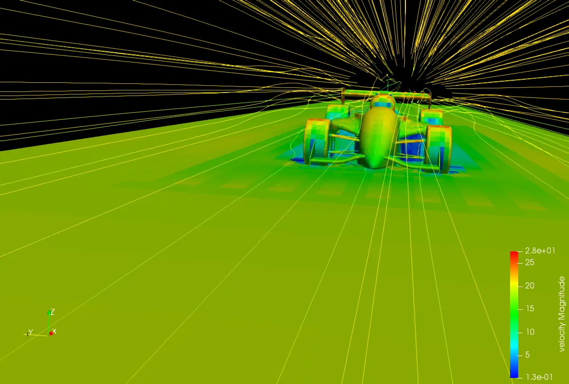
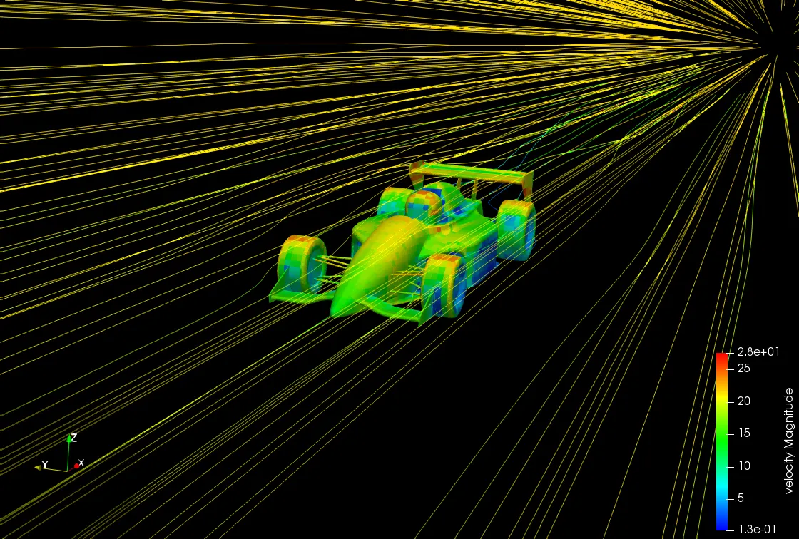
Stream Lines
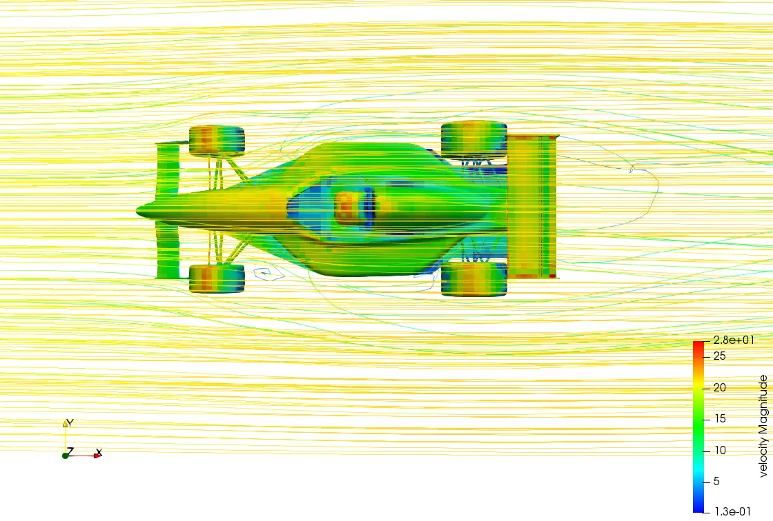
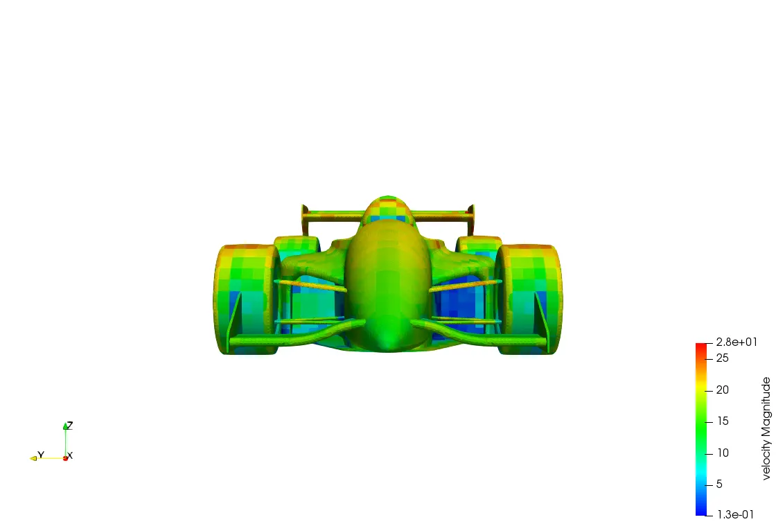
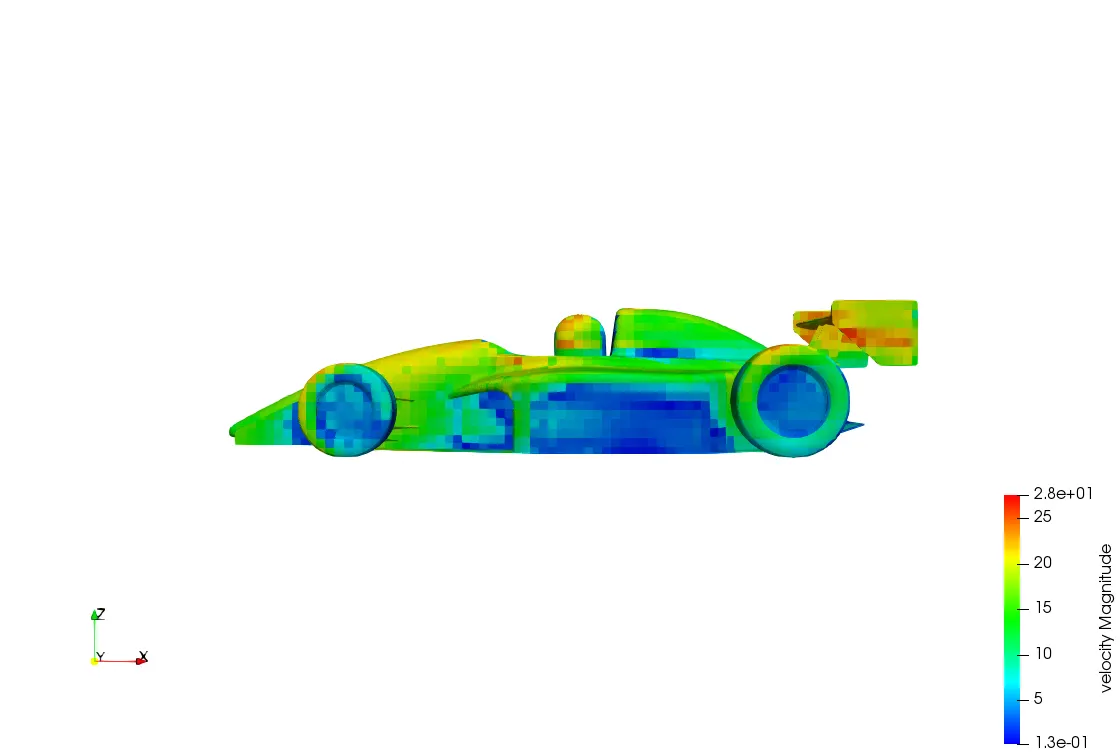
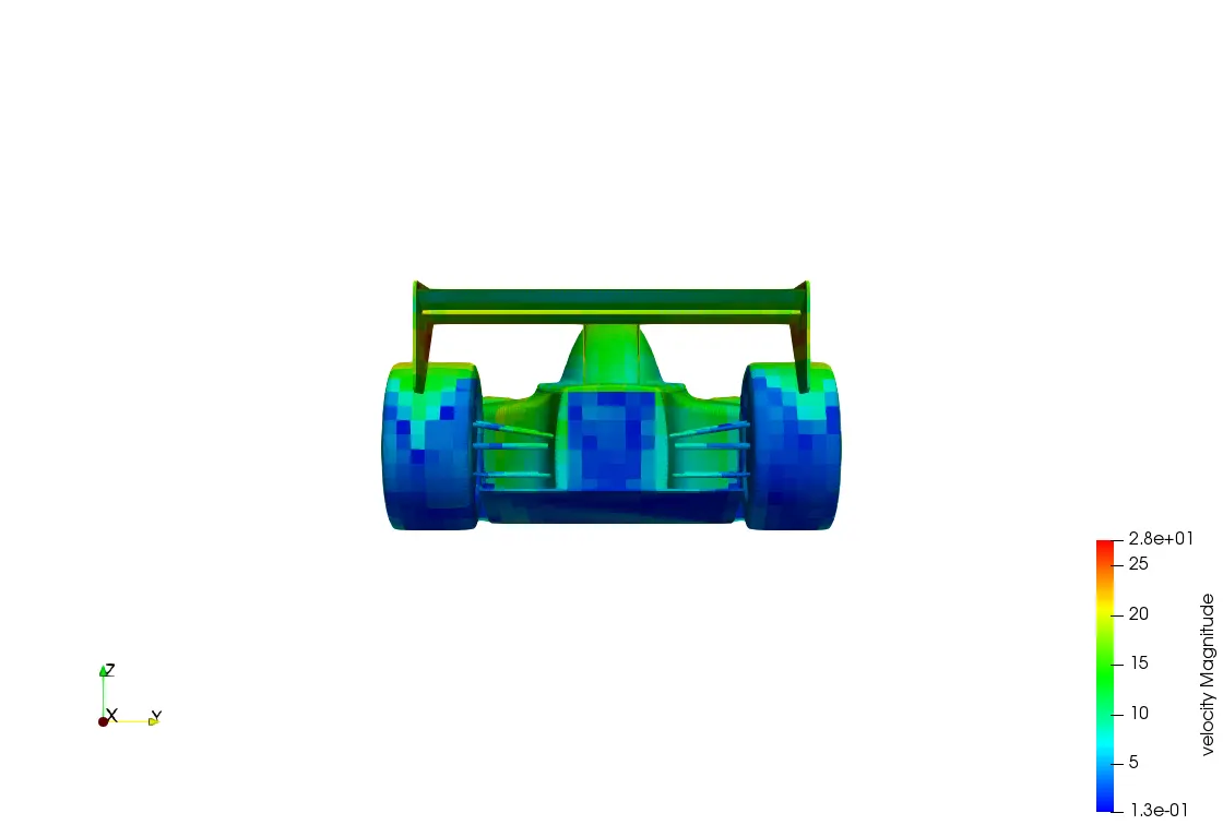
Y Plus
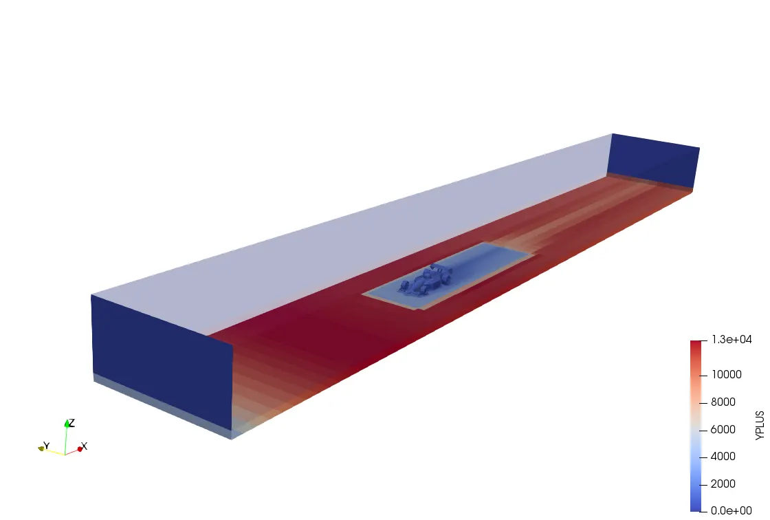
Y plus Contours
In this Y plus ranges from 1250 to 150.
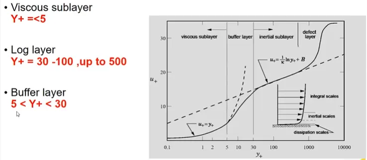
Turbulence is the state of chaotic and unstable fluid flow, just opposite of Laminar flow. Y plus(Y+) is the non-dimensional distance of the first cell from the wall.
Let's takes an example of a flat plate under zero pressure gradient and front left side the uniform velocity is coming to the plate. Firstly, it will be laminar flow, then after some disturbance, the region will be called as Transition Region, when the disturbance is growing too much the flow will change in Turbulent Flow. The boundary layer in the turbulent region will be called a turbulent boundary layer whereas in laminar it will be called the laminar boundary layer.
Reynold's Number Re is the ratio of Inertial force to the Viscous Force.
Viscous Sub Layer: Viscous stress term dominates
Buffer Layer: Transitional region
Log law Region: Reynolds shear stress term dominates
Velocity Contour:
Pressure Contour:
Line Plots
Mesh Count Plot
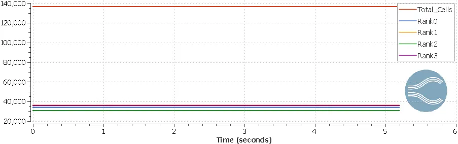
The total number of cells was found be to 140,000 and the case study was run using 4 processors that are represented by rank, the Base mesh was kept as 0.5 m and box embedding was given along the boundary embedding in order to refine the mesh near to major components to get a more accurate result. But due to less computational resources, these results were obtained with coarse type mesh.
Case Study 2
Case2 The condition was during turning
Racing track conditions - Lot of turns
- Average lap speeds - 45kmph
- 70% turns at 45 degrees
- 20% turns at 80 degrees
- 10% turns at 20 degrees
The car Model was rotated along Z-Axis
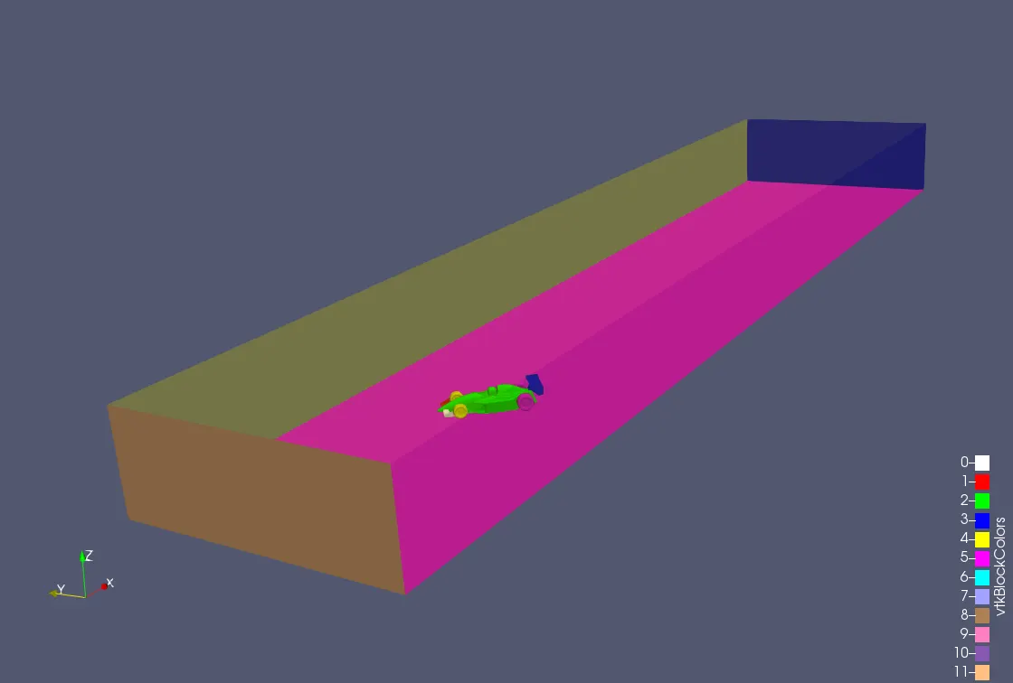
Mesh Model
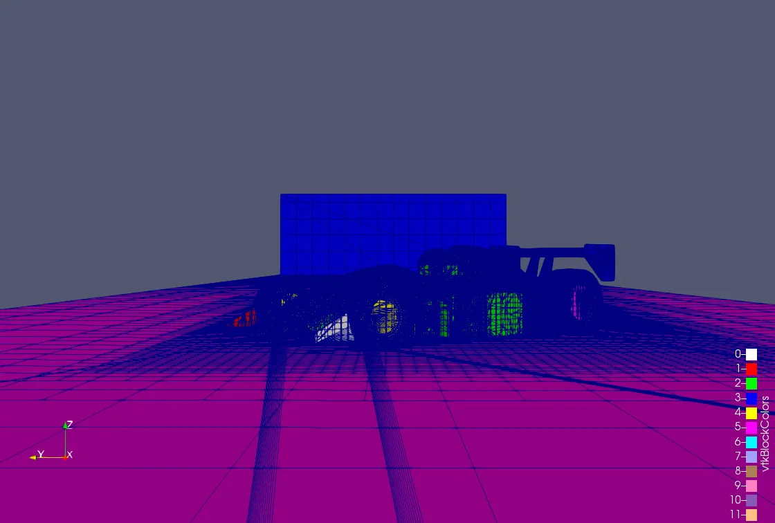
Contours
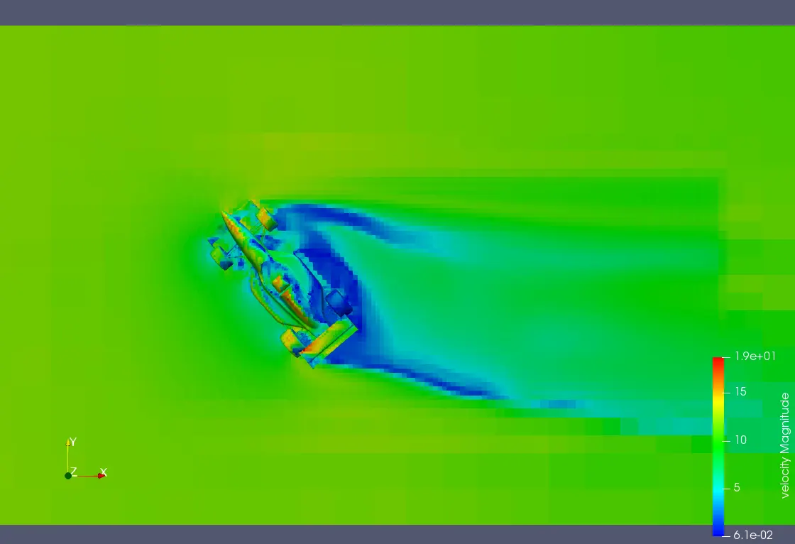
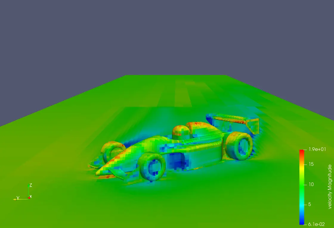
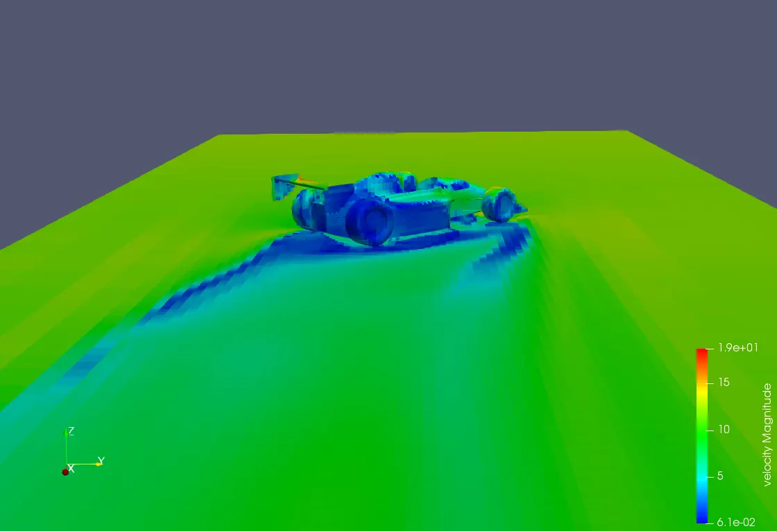
Velocity Contour
Observation
The velocity is low in the Windward side indicated in blue color and quite high in and around the region behind the car
The velocity is very low in the leeward side of the car and it extends to a vast region along the rear end of the car.
In this case, the recirculation zone is much higher as compared to case1 and is due to a larger area where pressure is low.
Interference
As the air that is the working fluid, in this case, strikes the car, it loses its kinetic energy which leads to a decrease in the velocity of the fluid in the windward side of the car.
the fluid that strikes on the car is diverted to the upper part of it, which adds up to the velocity of the fluid actually flowing above the car, thus an increase in velocity is noticed above the car due to the nice aerodynamics design of the car.
Some amount of flow is diverted to the side of the car it is due to the front wings of the car and front wings can be designed in such a way to generate the vortex so that it does not interrupt the wheel while the car is on the race track so as to reduce the tire drag.
There is a flow separation that can be seen behind the car near to rear wings it is due to change in air pressure on the NACA aerofoil that is being used in. Wings and there is also a drop in velocity that can be seen behind the car because of drop-in pressure. Due to flow separation a region of partial vacuum is formed in the leeward side of the car this leads to recirculation of air and this gives rise to vortex formation. These Vortexes tend to move along the wind direction and this entire region of low velocity in along the leeward side of the car is also called at Wake region.
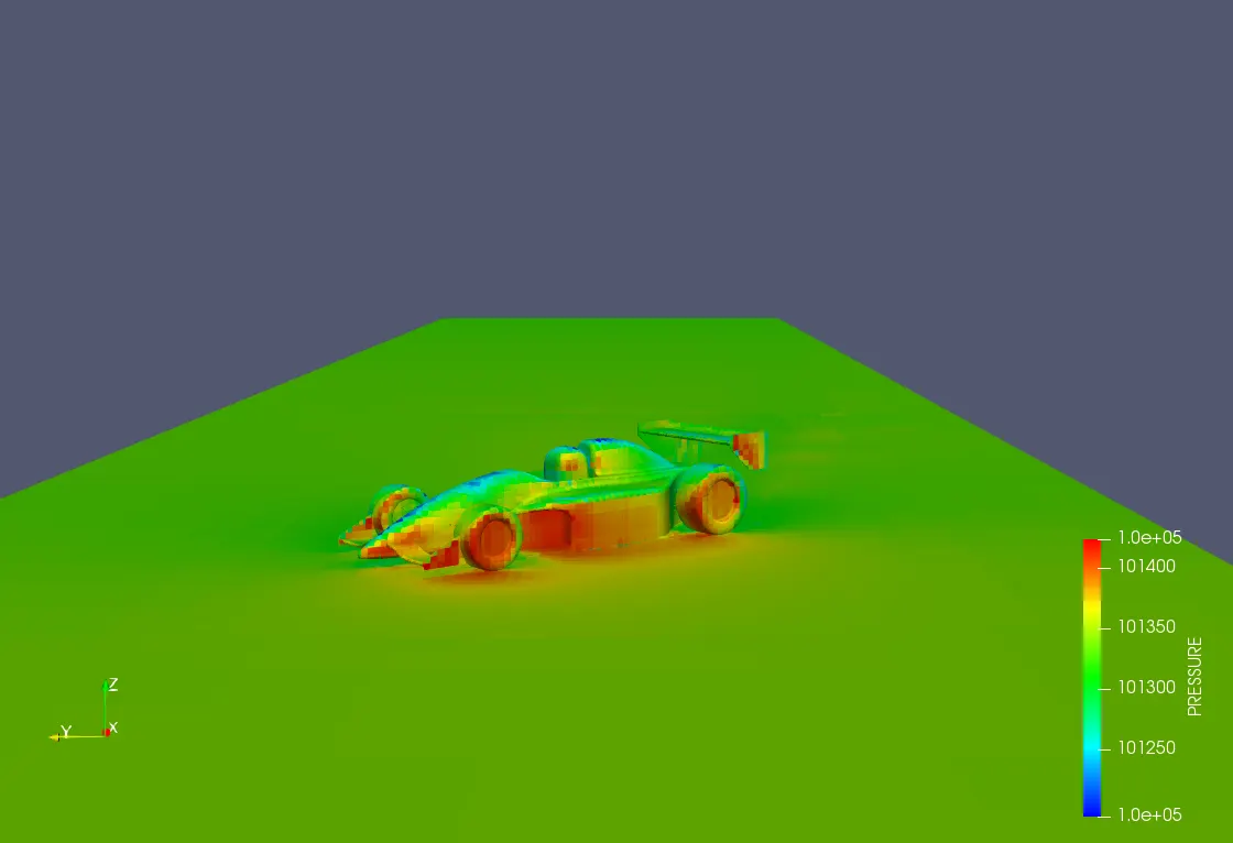
Pressure Contour
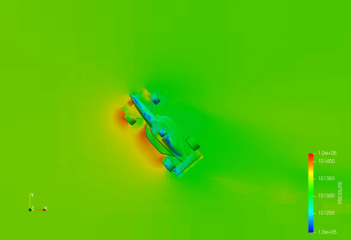
Observation
The pressure is very high in the windward side of the car indicated in the red region that is the left part of the car.
the part is very low along the axis of symmetry of the car indicated in dark blue and considerably low in the leeward side of the car.
Interface
As the Airstrikes the windward of the car, the kinetic energy is converted into pressure energy, hence, the pressure is very high here.
The low pressure along the axis of the car is accorded to hight velocity in this region.
the low pressure in the leeward side is attributed to the flow separation taking place there. As the partial vacuum forms and flow reversal takes place in the leeward side, it leads to low pressure in this region.
Stream Lines
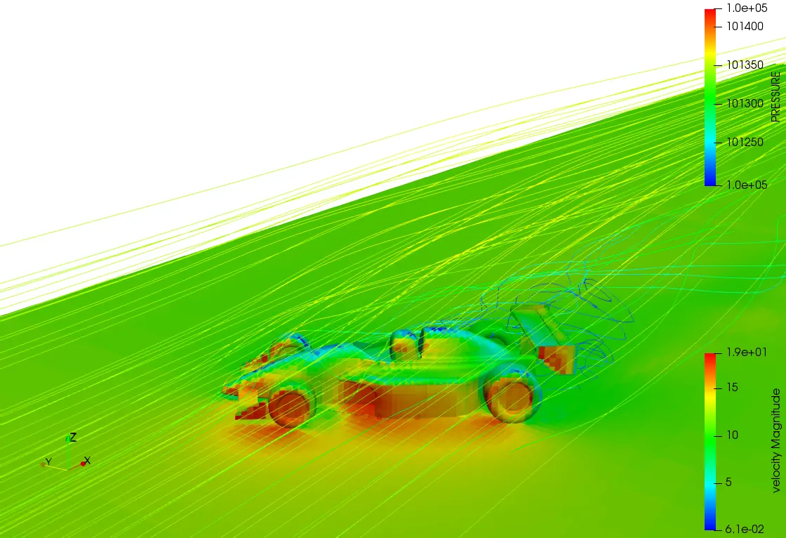
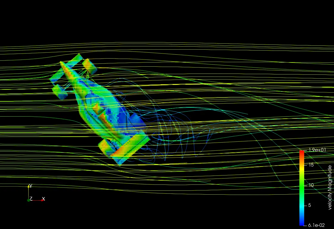
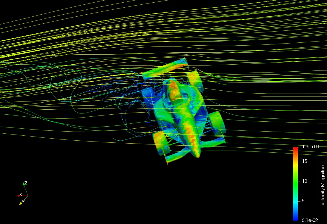
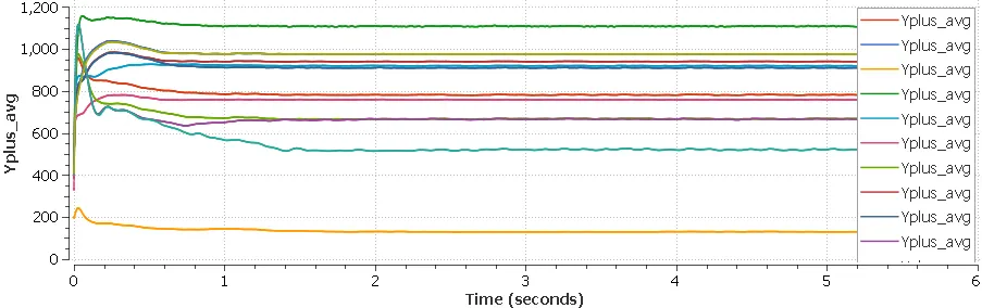
Y Plus
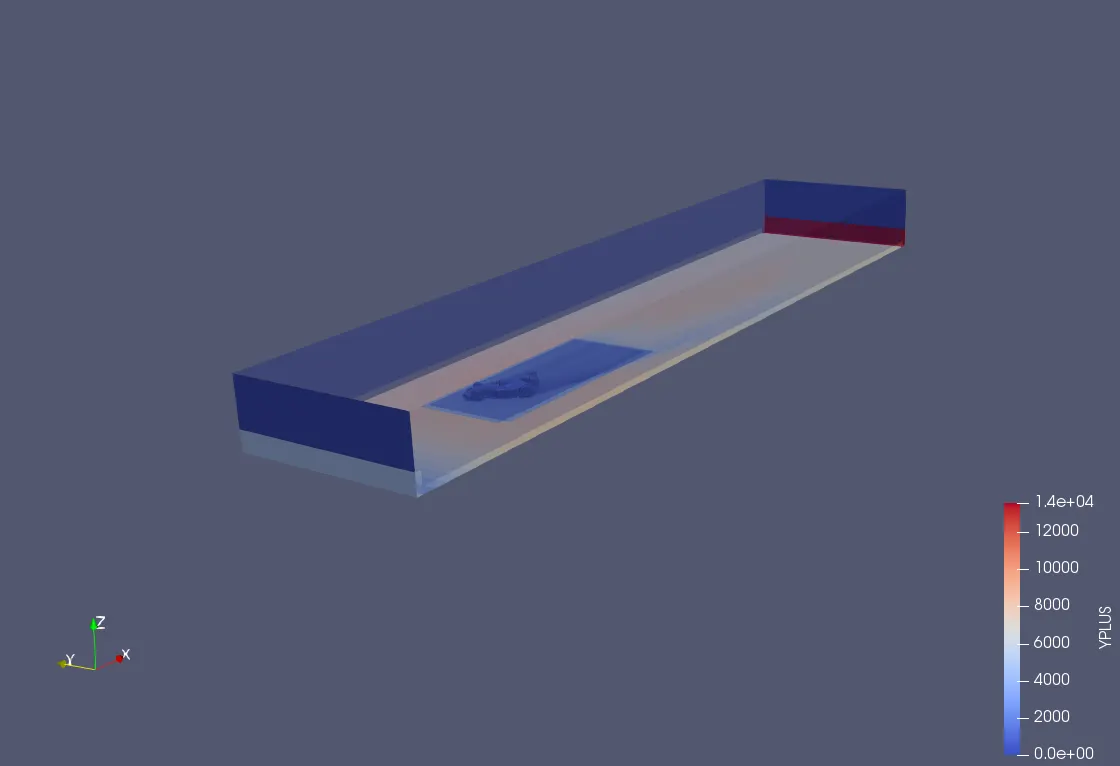
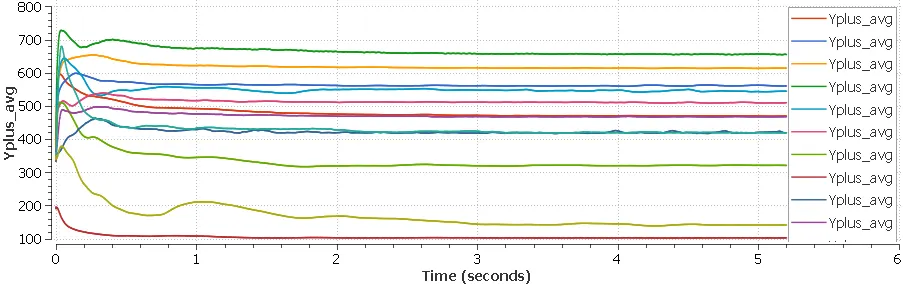
Y plus(Y+) is the non-dimensional distance of the first cell from the wall. For major components, Y+ ranges from 750 to 100.
Total Cell Count Plot
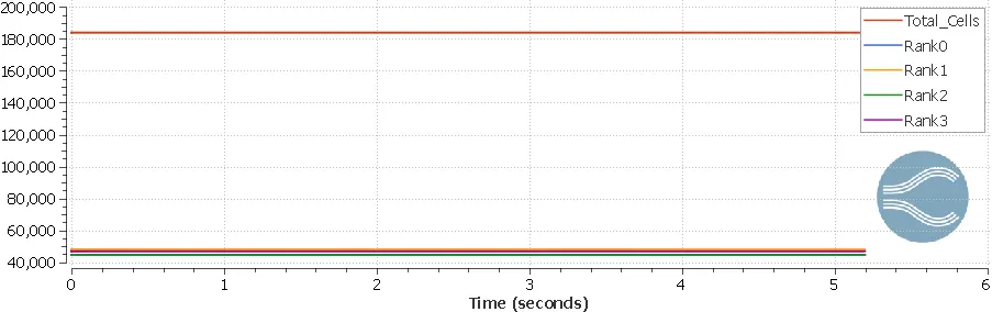
The total number of cells was found be to 170,000 and the case study was run using 4 processors that are represented by rank, the Base mesh was kept as 0.5 m and box embedding was given along the boundary embedding in order to refine the mesh near to major components to get a more accurate result. But due to less computational resources, these results were obtained with coarse type mesh.
----------------------------------------------------------------------------------------------------------------------
Finding the Coefficient of Lift and Drag using ParaView
ParaView is an important post-processing tool to visualize the results for the FSAE body. Various steps are followed in order to generate Lift and Drag force.
1. First the test.vtm files were imported in Paraview. The .Vtm was created using a converge studio using a post-processing dock.
2. The second step was to generate the FSAE body so that the "Extract Block" Filter was used to generate the FSAE body.
3. The third step was to generate the Surface of the FSAE body so a filter called "Extract surface" was used to extract surface for creating the surface normals.
4. Then the surface normals were created using the option in the filter.
5. Then the Lift and Drag force value was calculated using a Virtual calculator.
Lift Force(For single-cell) =PRESSURE*Normals_Z
Drag Force(For single-cell)=PRESSURE*Normals_X
6. Then the cell data were integrated using a filter called "Integrate Variable"
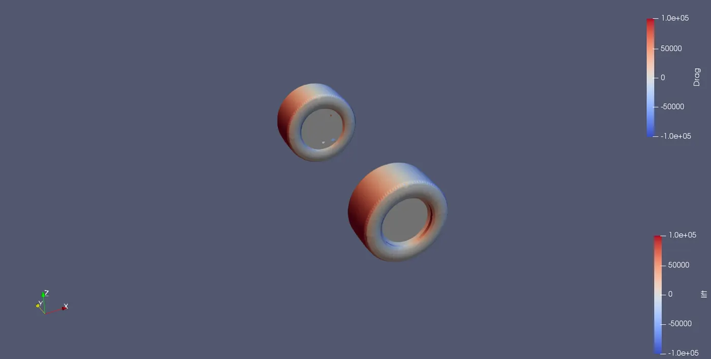
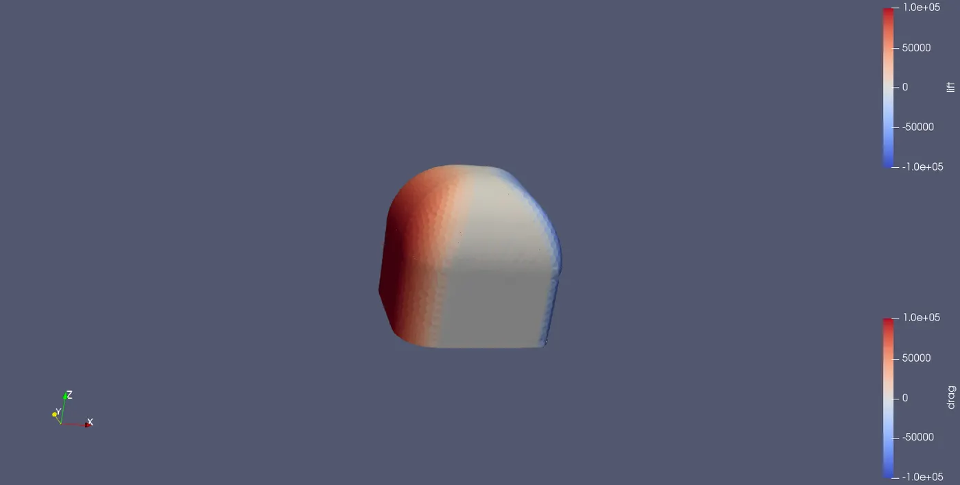
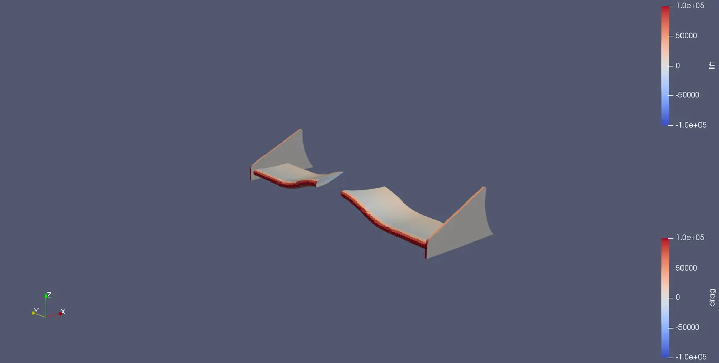
Case 1 Result
Front Suspension
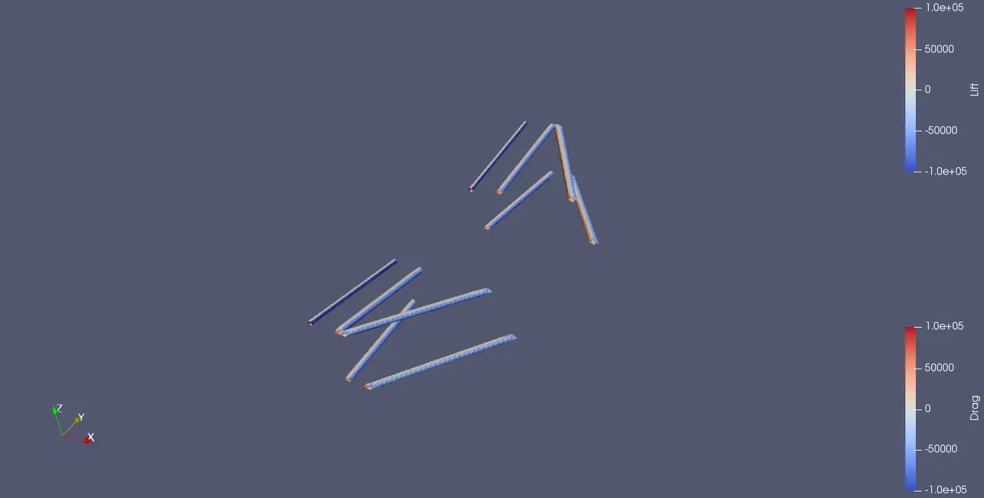
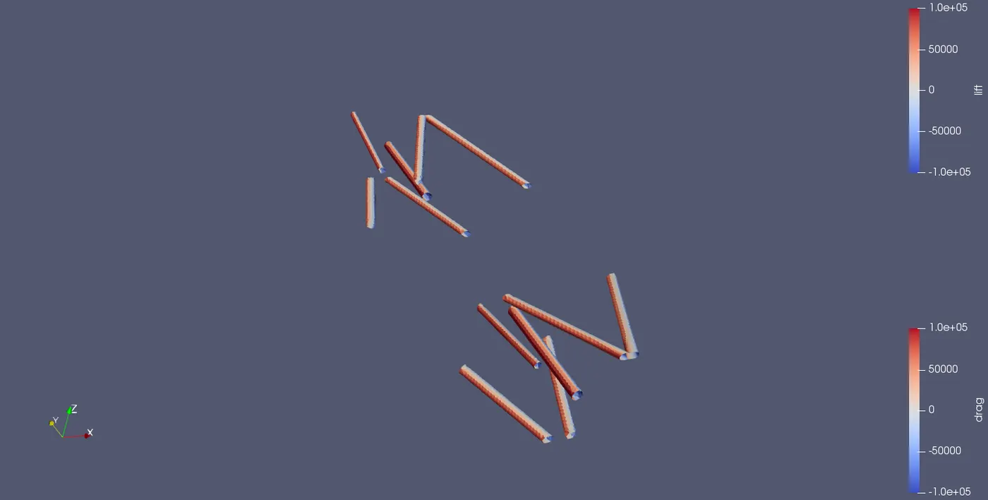
Rear Suspension
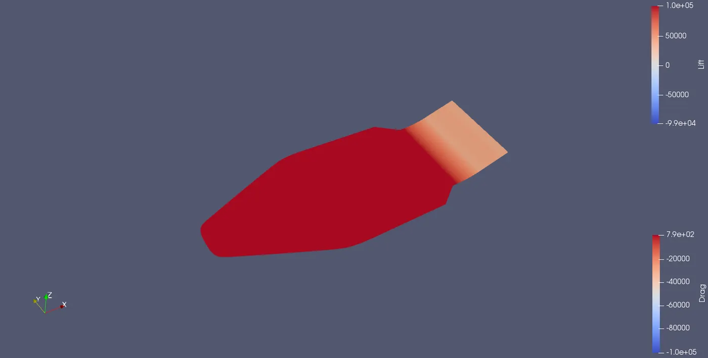
UnderTray
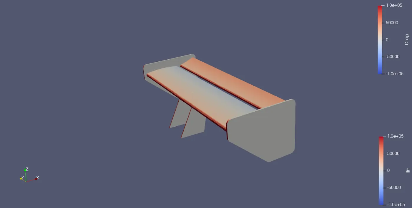
Rear Wing
Rear Wheel
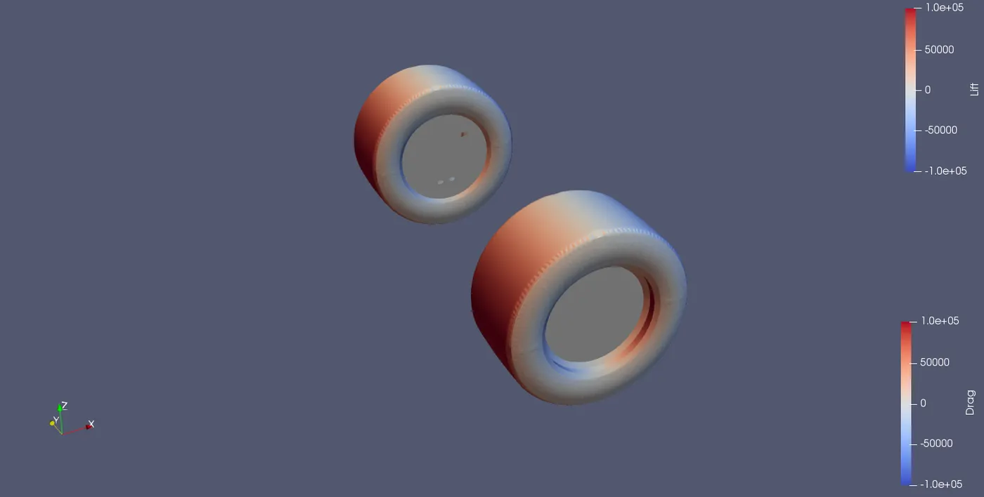
Front Wheel
Human
Front Wing
Body
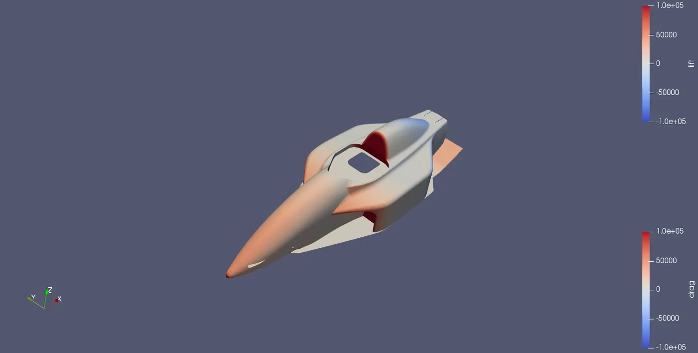
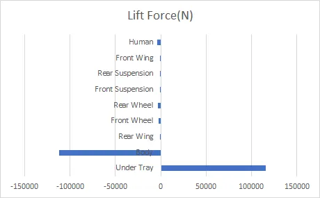
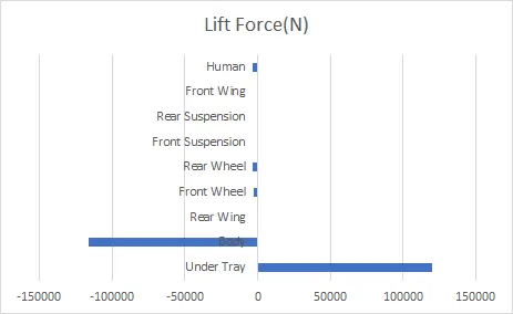
Lift Force
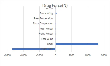
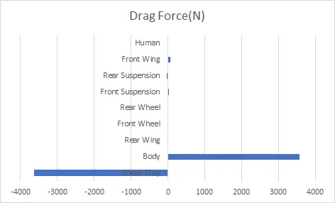
Drag Force
Over All Result For Drag and Lift Force
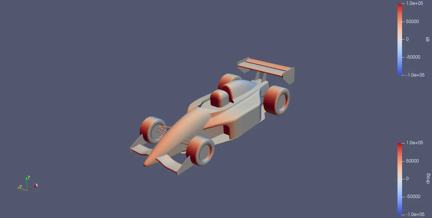
Result
| Lift Force | -5221.35N |
| Drag Force | 60.5816N |
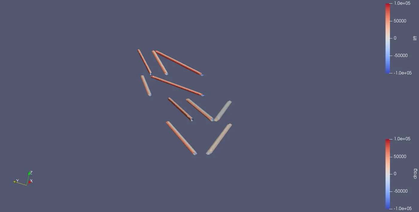
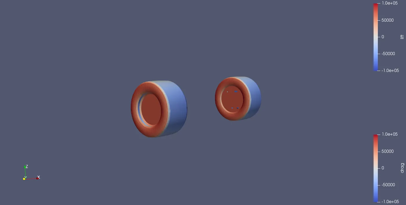
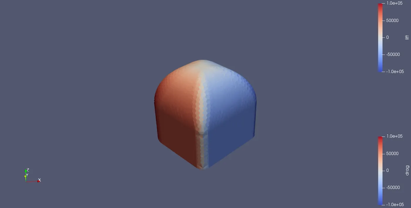
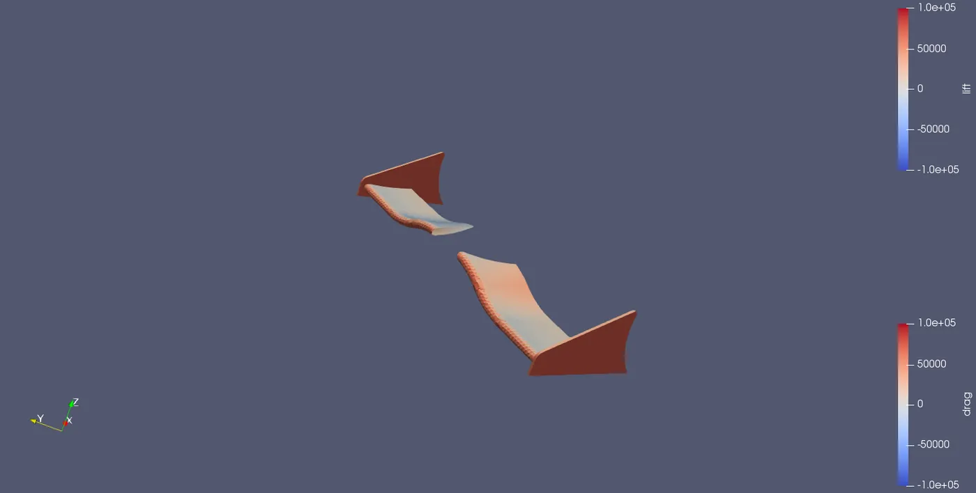
Case 2 Result:
Front Suspension
Rear Suspension
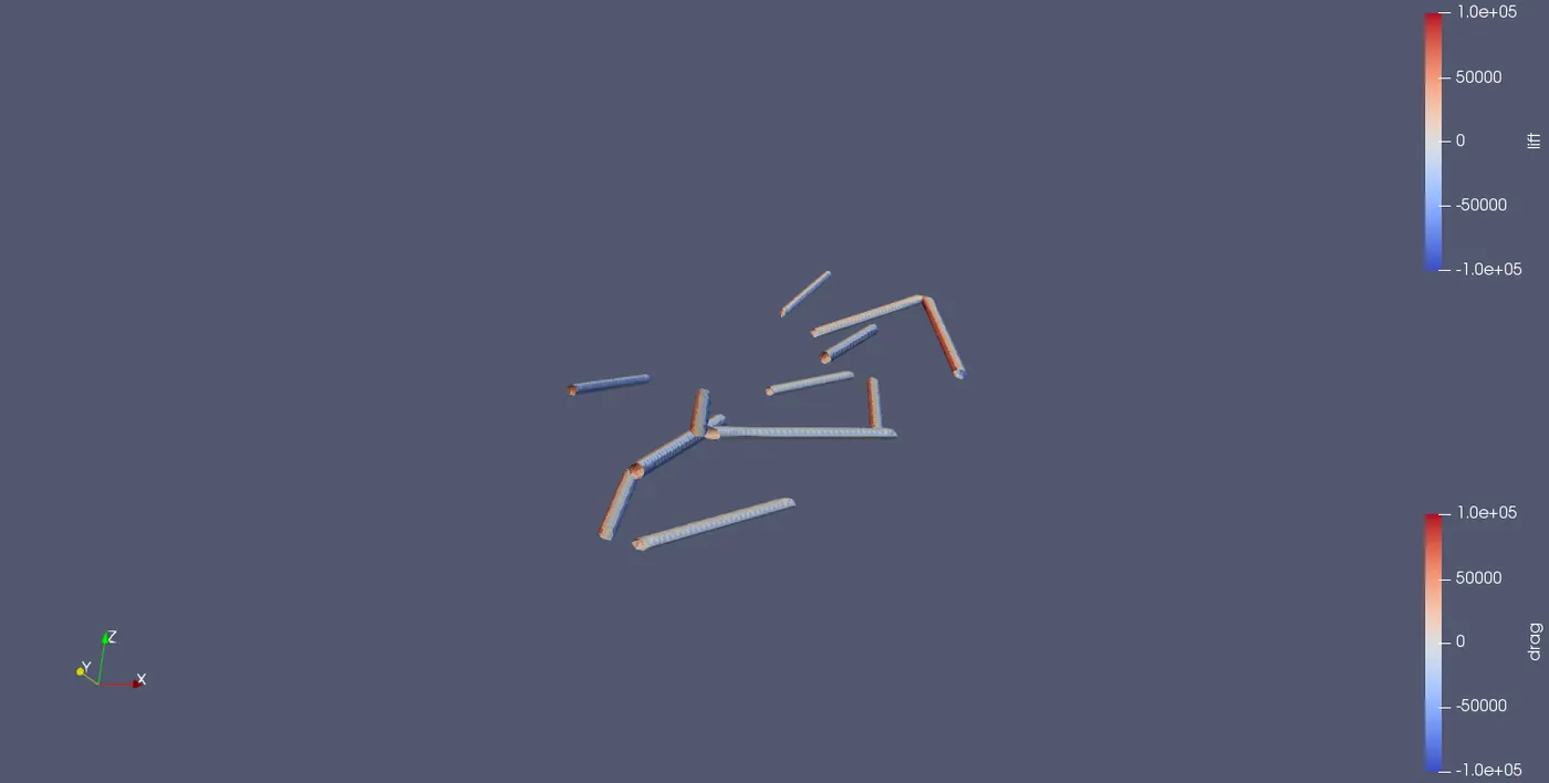
UnderTray
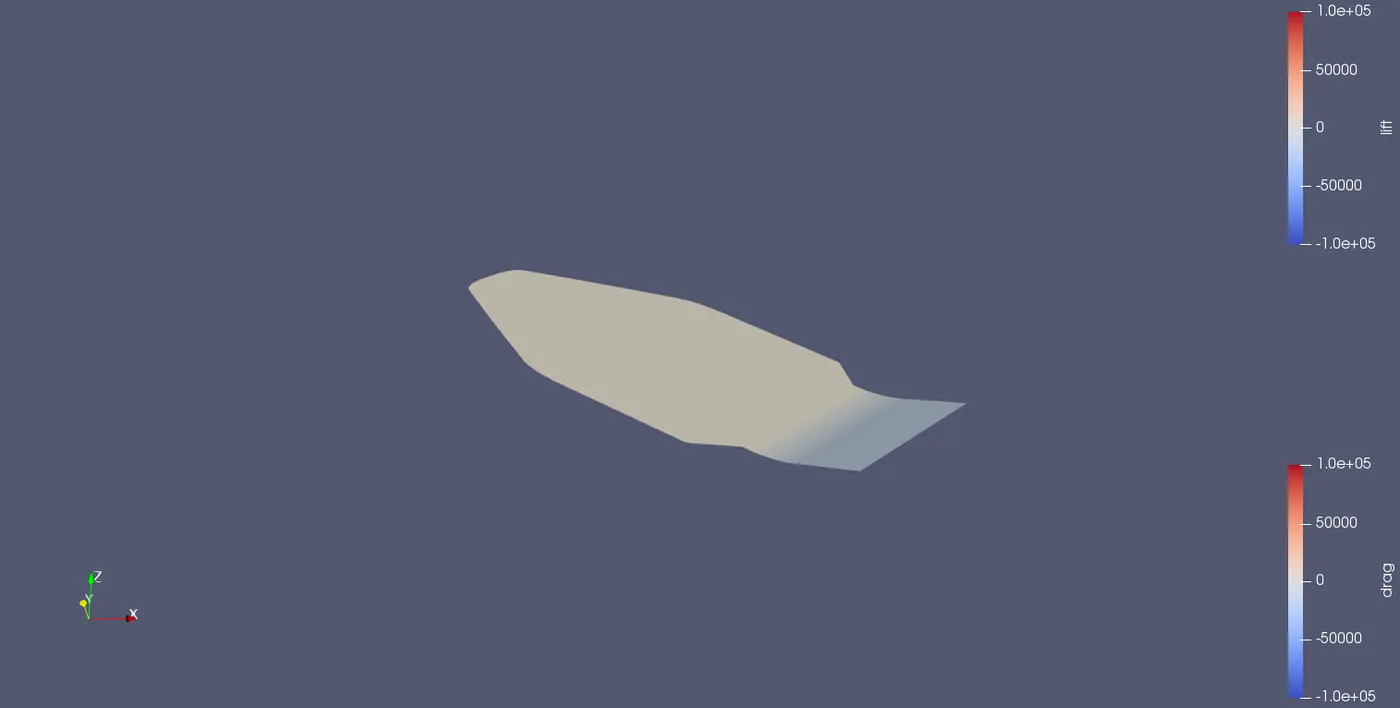
Rear Wing
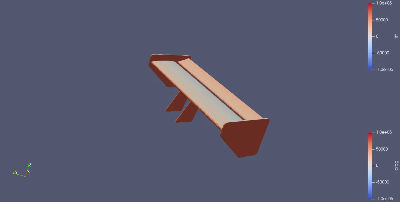
Rear Wheel
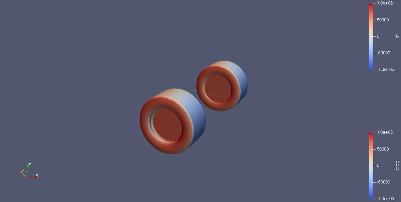
Front Wheel
Human
Front Wing
Body
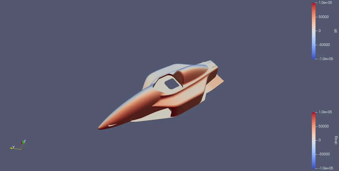
Lift Force
Drag Force
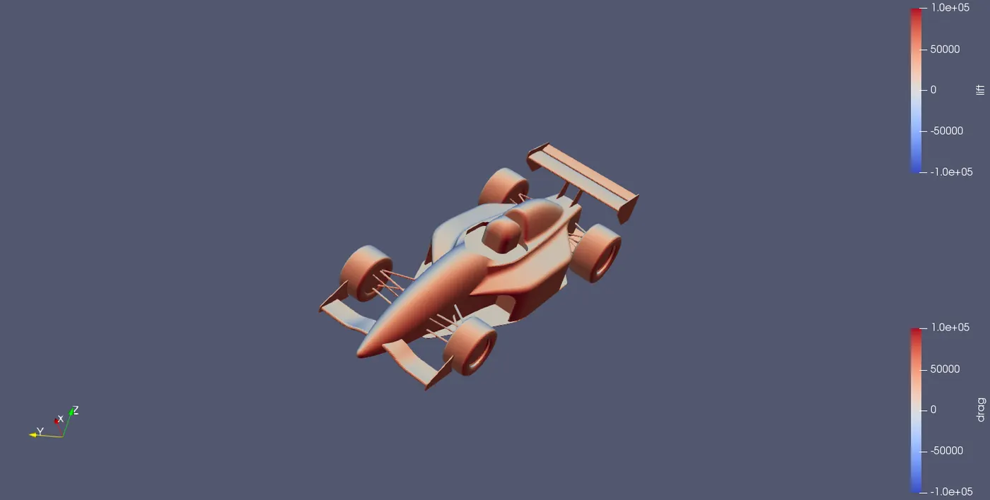
Over All Result For Drag and Lift Force
Result
| Lift Force | -5414.98N |
| Drag Force | -0.000914N |
Conclusion:
Case 1:
Observations:
The left front wing contributes to the major amount of the drag on the car. Also, the wheels and right front suspension contribute to a small amount of drag. The right front wing, rear suspension, combinatory force of body & underbody are found to push the vehicle in the direction of motion by producing -ve force.
Inference/ Recommendations:
As the pressure force acting on the left front wing is high, the drag force imparted by it on the car is quite higher. Similarly, a considerable amount of net pressure acts on the wheels, which produces some amount of drag. Unlike the previous, the right front suspension experiences drag as it belongs to the wake region(low-pressure region).
Case 2:
Observations:
The maximum amount of downforce is produced by the Human. A considerable amount of downforce is imparted by the wheels. The combinatory effect of the Body and the Underbody is found to offer a lift.
Inference/ Recommendations:
The downforce produced by human is accorded to the component of the resultant force acting on it due to pressure as shown below.
The file Can be downloaded from here: Case setup
The Excel sheet can be downloaded from here: Excel sheet