Literature review RANS derivation and analysis

Aim:

The major Objective was to apply Reynolds decomposition to the Navier Strokes equations and come up with Reynold's Stress. Understand the term, Reynolds Stress, and study the difference between turbulent viscosity and molecular viscosity.

Theory:

Turbulence :

Turbulence is the state of chaotic and unstable fluid flow, just opposite of Laminar flow. Y plus(Y+) is the non-dimensional distance of the first cell from the wall.

Let's takes an example of a flat plate under zero pressure gradient and front left side the uniform velocity is coming to the plate. Firstly, it will be laminar flow, then after some disturbance, the region will be called as Transition Region, when the disturbance is growing too much the flow will change in Turbulent Flow. The boundary layer in the turbulent region will be called a turbulent boundary layer whereas in laminar it will be called the laminar boundary layer.

Reynold's Number `Re` is the ratio of Inertial force to the Viscous Force.

`Re=(rho*V*l)/mu`

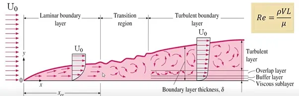
External Flow :`Re<5x10^5`Laminar Flow ||`Re>5x10^5` Turbulent Flow

Internal Flow : Re<2300 Laminar Flow || Re>4000 Turbulent Flow

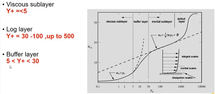
Viscous Sub Layer: Viscous stress term dominates

Buffer Layer: Transitional region

Log law Region: Reynolds shear stress term dominates

What is Reynold's Stress?

In fluid dynamics, the Reynolds stress is the component of the total stress tensor in a fluid obtained from the averaging operation over the Navier-Stokes equations to account for turbulent fluctuations in fluid momentum.

`T'_(uv)=-rho*u'*v'`

Turbulence Modeling Approaches :

Converge offers two turbulence modeling approaches

-Reynold-Averaged Navier Stokes (RANS)-Solves equation for an ensemble-averaged velocity field and the magnitude of the turbulent fluctuations.

-Large Eddy Simulation (LES)-Solves equations for a filtered time-dependent velocity field that represents large scale turbulence motion

Governing Equation for Boundary Layer

`(delu)/(delx)+(delu)/(dely)=0`------------Contunity equation

`u(delu)/(delx)+v(delu)/(dely)=-1/rho*(delp)/(delx)*nu*((del^2u)/(delx^2)+(del^2u)/(dely^2))`-----------------------X-momentum Equation

`u(delv)/(delx)+v(delv)/(dely)=-1/rho*(delp)/(delx)*nu*((del^2v)/(delx^2)+(del^2v)/(dely^2))`-----------------------Y-momentum Equation

`u(delT)/(delx)+v(delT)/(dely)=alpha((del^2T)/(delx^2)+(del^2T)/(dely^2))`----------------------------------------------Energy Equation

If we take the original governing equation and we integrate over a small time step and we have a huge number of computational cells, then we don't need any turbulence model. But this approach is impractical so that is why people are using the turbulence mode

We will use these governing equation and we will integrate over a time that is much larger than the turbulence time scale. This is called the Averaging process we apply Reynold Decomposition process, we obtain an original set of the equation that is called RANS.

Reynold Decomposition:

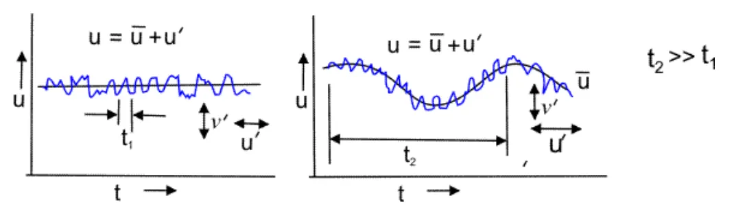
In this process, we decompose a function into a mean and fluctuating function.

`u(x,y,z,t)=baru(x,y,z)+u'(x,y,z,t)`

`v(x,y,z,t)=barv(x,y,z)+v'(x,y,z,t)`

`w(x,y,z,t)=barw(x,y,z)+w'(x,y,z,t)`

Here,

u=instantaneous velocity

`baru`=Average Velocity

u'=Fluctuation Velocity

The mean time average velocity is a function of space while the fluctuating velocity is the function of space and time both.

Now, On integrating Average velocity from 0 to intT

`baru(x,y)=(1/t_i)∫_0^(t_i)u(x,y,t)dt`

`barv(x,y)=(1/t_i)∫_0^(t_i)v(x,y,t)dt`

We know that on integrating the fluctuating velocity its value is always Zero and here is the proof

`1/t_i∫_0^(T)u'(x,y,t,z)dt=0`

To prove this we again used Reynold decomposition principle.

`baru=1/Tint_0^T barudt+1/Tint_0^T u'dt`

`cancelbaru=cancelbaru+1/Tint_0^Tbaru dt`

So We get,

`1/Tint_0^Tbaru dt=0`

Applying Reynold's Decomposition on Continuity Equation

`(delu)/(delx)+(delv)/(dely)=o`--------------------------contuinity equation

Applying Reynold's Decomposition,

`(del(overlineu+u'))/(delx)+(del(overlinev+v'))/(delv)=0`

On splitting, We get

`1/Tint(deloverlineu)/(delx)dt+1/Tint(delu')/(delx)dt+1/Tint(deloverlinev)/(dely)dt+1/Tint(delv')/(dely)dt=0`

We know that Time average of fluctuating is always Zero.

`1/Tint(deloverlineu)/(delx)dt+cancel(1/Tint(delu')/(delx)dt)+1/Tint(deloverlinev)/(dely)dt+cancel(1/Tint(delv')/(dely)dt)=0`

`1/T(deloverlineu)/(delx)intdt+1/T(deloverlinev)/(dely)intdt=0`

Applying Limits & Intregrating

`1/T(deloverlineu)/(delx)int_o^Tdt+1/T(deloverlinev)/(dely)int_0^Tdt=0`

`(deloverlineu)/(delx)[T-o]/T+(deloverlinev)/(dely)[T-o]/T=0`

We finally get,

`(deloverlineu)/(delx)+(deloverlinev)/(dely)=0`

That means the Time Avaerge satisfy the Continuity equation.

Applying Reynold's Decomposition on Momentum Equation

`rho[(delu)/(delt)+u(delu)/(delx)+v(delu)/(dely)]=-(delp)/(delx)+mu(del^2u)/(dely^2`

`[(delu)/(delt)+u(delu)/(delx)+v(delu)/(dely)]=1/rho[-(delp)/(delx)+mu(del^2u)/(dely^2)]`

Replacing `mu/rho=nu` by Kinematic viscocity

adding an extra term on left side

`[(delu)/(delt)+u(delu)/(delx)+v(delu)/(dely)]+u[(delu)/(delx)+(delv)/(dely)]=-1/rho(delp)/(delx)+nu(del^2u)/(dely^2)`

On Simplifying

`[(delu)/(delt)+2u(delu)/(delx)+v(delu)/(dely)+u(delv)/(dely)]=-1/rho(delp)/(delx)+nu(del^2u)/(dely^2)`

Using Produt Rule by substituting the Cross product

`[(delu)/(delt)+2u(delu^2)/(delx)+(deluv)/(dely)]=-1/rho(delp)/(delx)+nu(del^2u)/(dely^2)`

Applying Reynold Decomposition

`1/Tint_0^T[(del(overlineu+u'))/(delt)+2u(del(overlineu+u')^2)/(delx)+(del(overlineu+u')(overlinev+v'))/(dely)]=1/Tint_0^T[-1/rho(delp)/(delx)+nu(del^2u)/(dely^2)]`

`1/Tint_0^T[(deloverlineu)/(delt)dt+(delu')/(delt)dt+(deloverlineu)/(delx)dt+(delu')/(delx)dt+2(deloverlineu*u')^2/(delx)dt+(deloverlineuoverlinev)/(dely)dt+(delu'v')/(dely)dt+(delu'v')/(dely)dt+(delu'overlinev)/(dely)dt]=1/Tint_0^T[-1/rho(deloverlineP)/(delx)dt-1/rho(delP')/(delx)dt+nu(del^2u')/(dely^2)dt+nu(del^2overlineu)/(dely^2)dt]`

`1/Tint_0^T[(deloverlineu)/(delt)dt+cancel((delu')/(delt)dt)+(deloverlineu)/(delx)dt+(delu')/(delx)dt+cancel(2(deloverlineu*u')^2/(delx)dt)+(deloverlineuoverlinev)/(dely)dt+cancel((delu'v')/(dely)dt)+(delu'v')/(dely)dt+cancel((delu'overlinev)/(dely)dt)]=1/Tint_0^T[-1/rho(deloverlineP)/(delx)dt-cancel(1/rho(delP')/(delx)dt)+cancel(nu(del^2u')/(dely^2)dt)+nu(del^2overlineu)/(dely^2)dt]`

`[(deloverlineu)/(delt)+(deloverlineu^2)/(delx)+(deloverlineuoverlinev)/(dely)]=-1/rho(deloverlineP)/(delx)+nu(del^2overlineu)/(dely^2)-1/Tint_0^T(del(u')^2)/(delx)dt-1/Tint_0^T(del(u'v'))/(dely)dt`

`[(deloverlineu)/(delt)+(deloverlineu^2)/(delx)+(deloverlineuoverlinev)/(dely)]=-1/rho(deloverlineP)/(delx)+nu(del^2overlineu)/(dely^2)-1/Tint_0^T(del(u'v'))/(dely)dt`

`[(deloverlineu)/(delt)+(deloverlineu^2)/(delx)+(deloverlineuoverlinev)/(dely)]=-1/rho(deloverlineP)/(delx)+1/rhodel/(dely)(mu(deloverlineu)/(dely)-rho*u'*v')`

In the above equation `rho*u'*v'` represents as added stress on the fluid.

What is Turbulent Viscosity? How is it different from Molecular Viscosity?

The turbulent viscosity is also called as eddy viscosity. In the study of turbulence in fluids, a common practical strategy is to ignore the small-scale vortices (or eddies) in the motion and to calculate a large-scale motion with an effective viscosity, called the "eddy viscosity", which characterizes the transport and dissipation of energy in the smaller-scale flow (see large eddy simulation). In contrast to the viscosity of the fluid itself, which must be positive by the second law of thermodynamics, the eddy viscosity can be negative.

Molecular viscosity is the same as viscosity. The Coefficient of Molecular Viscosity is the same value as dynamic viscosity. Molecular viscosity is the transport of mass motion momentum solely by the random motions of individual molecules not moving together in coherent groups. Molecular viscosity is analogous in laminar ow to eddy viscosity in a turbulent flow.

The dynamic viscosity or molecular viscosity is a macroscopic fluid property, you can think of it as what distinguishes honey and water. And the eddy viscosity or turbulent viscosity is a flow property emerging from the increased momentum transport through the flow field due to turbulent velocity fluctuations.