Conjugate Heat Transfer Simulation
Conjugate Heat Transfer Simulation
Aim:
The major objective of this project was to Simulate an Aluminium cylindrical tube for the Conjugate Heat Transfer problem using Converge CFD and Post-processing the result using ParaView to study the change of result when the major parameter is changed like grid size.
Introduction:
The report contains a detailed description of the Conjugate Heat Transfer problem using converge CFD software, solving it using CYGWIN, and post-processing the result using ParaView. Various steps are discussed in this report while making a case set up for this case study. This report contains a detailed description of the case study with grid sizing, line plots, the effect of Superheating parameter, and contours.
Conjugate Heat Transfer (CHT) is when heat transfer occurs simultaneously within and between fluid and solid regions.
-The predominant mode of heat transfer in a fluid is convection.
-The predominant mode of heat transfer in a Solid is conduction.
Converge solves the fluid heat transfer using the energy equation.
converge solve the solid heat equation using the solid heat equation.
`C_p*rho((dT)/dt)=nabla.(k*nabla t) +Sh`
CHT Modeling Setup
There are several steps to setting up a CHT simulation
1.Define fluid and solid material and their physical properties
2.Configure the fluid and solid regions
3. Assign region to streams.
4. Use appropriate boundary conditions for the boundaries that separated different regions.
5. Select the time control method.
6. Set up post-processing.
Super-cycling
Super-cycling is a method used by CONVERGE Studio in the case of conjugate heat transfer problems with solid and liquid regions.
The integral problem here is that both solvers cannot run at the same speed since solving in the fluid domain is much faster owing to the time scale difference for heat transfer in liquids as compared to solids. This causes problems during the solution given that the solid side solver would not have reached a steady-state/convergence in the time the liquid solver does. This is where the concept of super-cycling can be used.
The basic idea of super-cycling is that the solver for the fluid domain is paused until the solver for the solid domain converges.
Calculation of Grid Size
Reynolds Number Re=7000
The density of Air(at 300k)=`rho=1.766 (kg)/m^3`
Dynamic Viscosity(at 300k)=`mu=0.00001846(kg)/(ms)`
Kinematic Viscosity=`mu/rho=1.56893E-0.5m^2/s`
Pipe Inner Diameter d=0.03m
Pipe Outer Diameter D=0.04m
Average Flow Velocity=`(Re.mu)/(rho.d)=3.66m/s`
Skin friction drag coefficient=`Cf=0.0576*Re^(-1/5)=0.00980399`
Wall Shear Stress=`T_w=Cf.((rho.v^2)/2)=0.077296708N/m^2`
Frictional Velocity=`ut=sqrt(tw)/rho=0.256310311m/s`
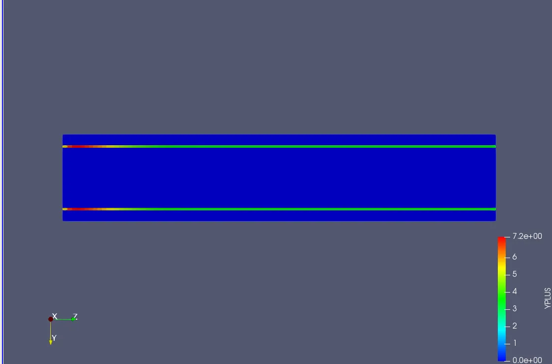
Assuming the desired `y+ =32`
Then first cell center to boundary distance=`y+*v/(ut)=0.001958785m`
Cell Size=`2*(0.001958)*1000=3.92mm~~4mm`
1.Geometry Creation
First of all, The geometry was created using the converge studio for that two-cylinder that was created with a different radius but with the same center. Then the circular patches were removed from both the cylinder, then two patches were created using the inner edge and the outer edge of the cylinder then was named as a solid side in boundary naming. The inlet was created using the fill surface and the same for an outlet for inner cylinder.
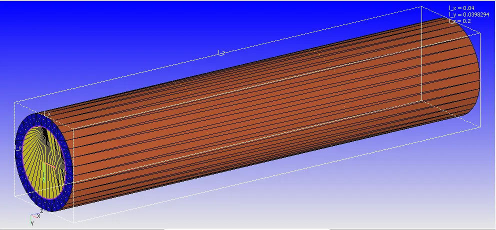
The Dimension of the Cylinder is Dx=0.04m, Dy=0.04m, Dz=0.2m.
Pipe Inner Diameter d=0.03m
Pipe Outer Diameter D=0.04m
All the normal vector were pointing out for this geometry, so we wanted it to point inside and normal to each surface. Normals point the direction of the fluid region generally. The command "Transform" was used to make the normal inside pointing the direction of the fluid region.
The Geometry was a check for if the geometry has any open surface.
2.Boundary Creation
After creating the Geometry, The Boundry tag was created along with different boundary id and coloring. A total of 5 different boundaries tag was created for so many different split triangles of the duct with each face split into multiple triangles. To create the boundaries naming, the "Boundary" command in the "Geometry" dock was used, and then the faces were appointed to appropriate tags along with id.
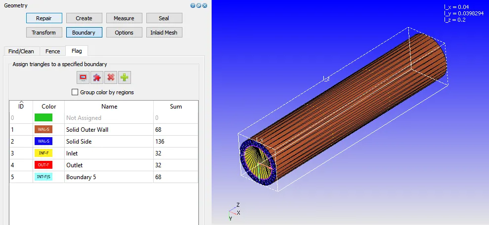
The five different boundaries were Inlet, Outlet, Solid outer wall, Solid Side, and Boundary 5(Interface).
3.Case-Study Setup
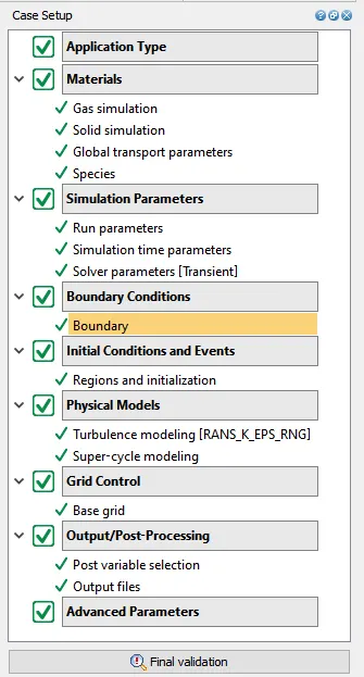
The various parameter was considered while setup this case study. The case study setup dock was used to set up the problem which appears on the right-hand side of the converge studio.
3.1 Application Type:
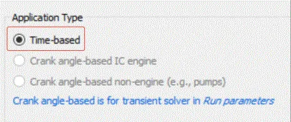
In order to run a steady-state simulation, firstly, under the Application type in the setup tree, a "Time-based" simulation must be selected.
3.2 Materials:
Under the material tab "Gas simulation" was selected and "Air" as a predefined mixture.
Gas: Air
Global Transport Parameters: Fixed value
by default, the following value is considered.
Prandtl Number : 0.9
Schmidt Number : 0.78
Species: Oxygen-O2 & Nitrogen-N2
Species and Solid Simulationwere selected for this problem.
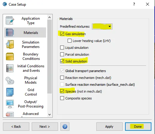
For Solid Simulation, The aluminum metal was selected out of many predefined metals.
3.3 Simulation Parameters:
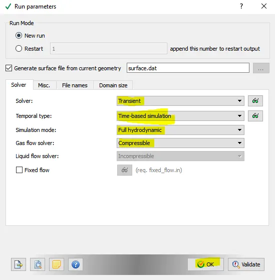
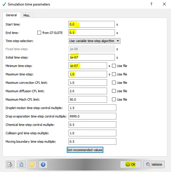
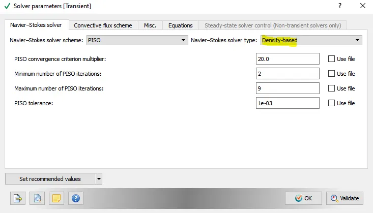
The Transient solver was selected for running this case study along with a "Density-based" solver.
3.4: Boundary Conditions:
In this tab, The volumetric region and physics for each boundary were defined.
| Boundary_Name | Boundary_Type | Paramter_Defined | Boundary ID |
| 1.Inlet | Inflow | 3.66m/s at 300k flow is Air | 3 |
| 2.Outlet | OutFlow | 101325 Pa | 4 |
| 3.Solid Outer Wall | Wall | Heat Flux=-10000W/m^2 | 1 |
| 4.Solid Side | Wall |
Slip |
2 |
| 5.Boundary 5 | Interface | law of Wall | 5 |
3.5: Initial Conditions and Events:
Volumetric Region was created for fluid in order to assign this to all the fluid flow boundary tag.
Species:- O2 (0.23) & N2 (0.77)
Pressure :101325Pa
Temperature:300K
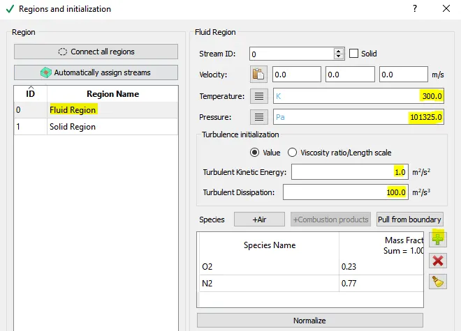
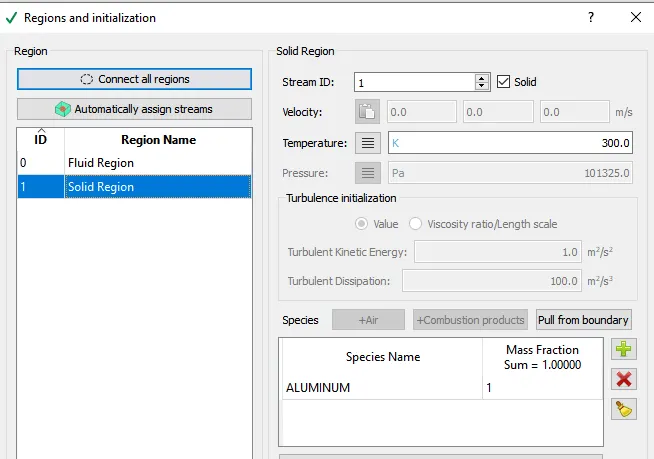
3.6: Physical Models:
A turbulent model was selected out of so many models.
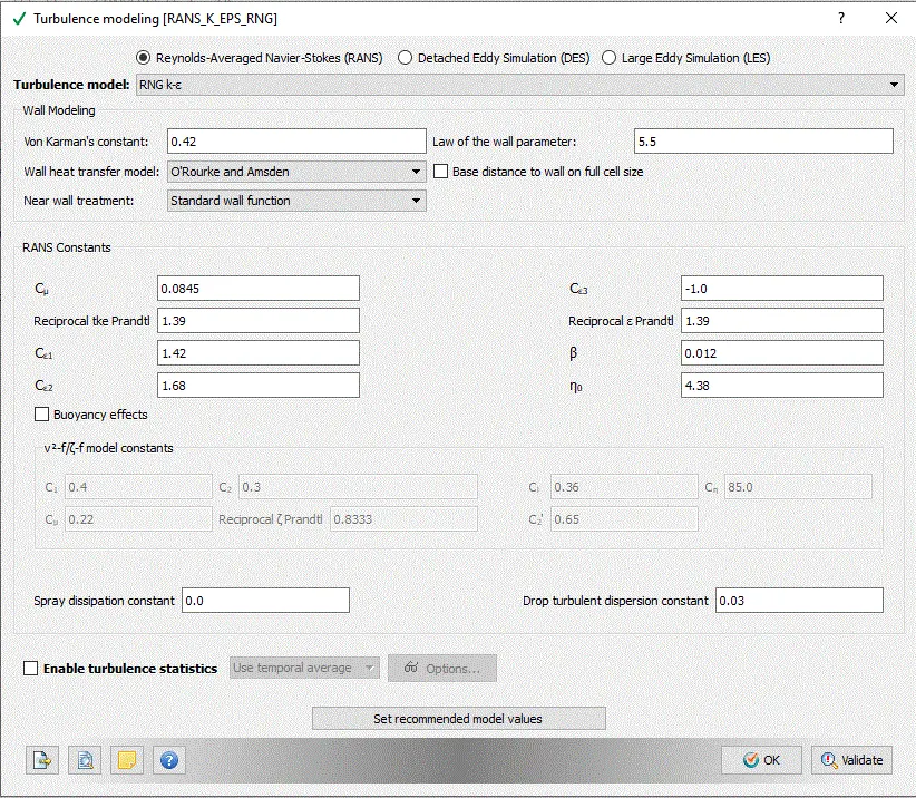
For SuperHeating Parameters
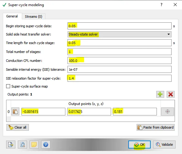
3.7: Grid Control:
The case study was run using a 3 different grid size. So different case study was set up in order to study the effect of value when the mesh is more refined.
The Adaptive mesh refinement was selected
Base mesh sizes are,
| S.No. | Dx(m) | Dy(m) | Dz(m) | Speed(m/s) |
| 1 | 0.004 | 0.004 | 0.004 | 3.66 |
| 2 | 0.003 | 0.003 | 0.003 | 3.66 |
| 3 | 0.002 | 0.002 | 0.002 | 3.66 |
3.7 Output/Post-Processing:
Post-Variable Selection- Existing value
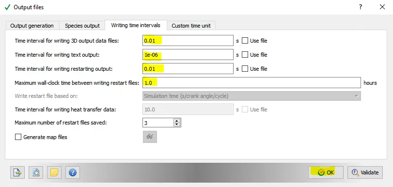
Output Files- Time interval for writing 3D output files-0.01 s
The time interval for writing restart files -0.01s
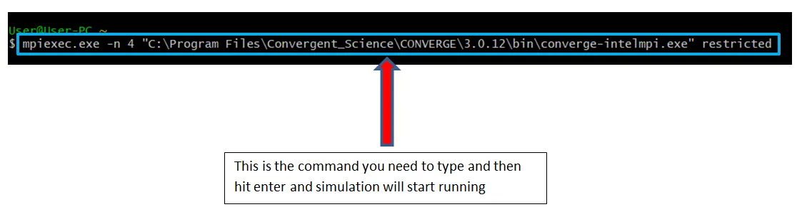
The case study was solved using CYGWIN and the post-processing was done in ParaView.
Simulation Result:
Grid Dependence Test
Case Study 1: Mesh Size 0.004m :
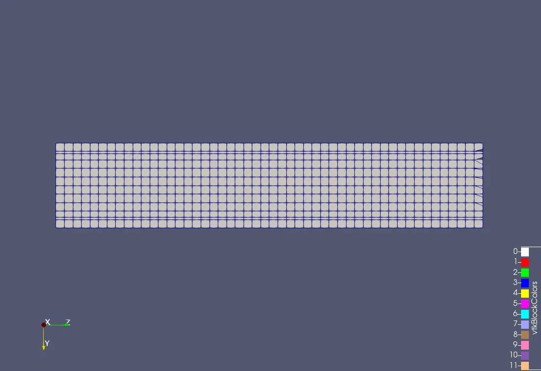
Generated Mesh:
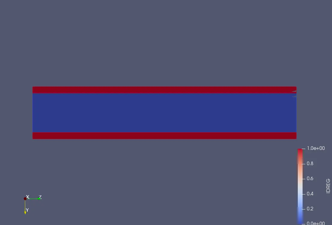
IDREG:
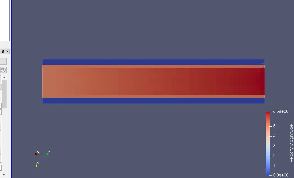
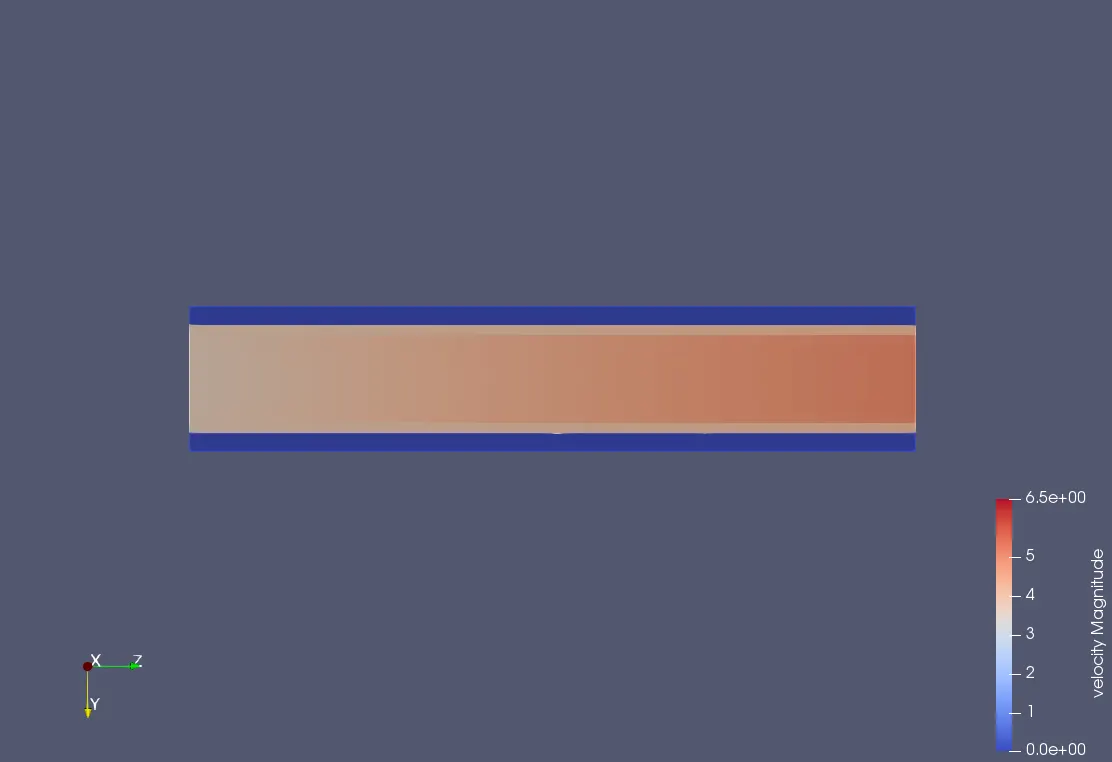
Velocity Contour:
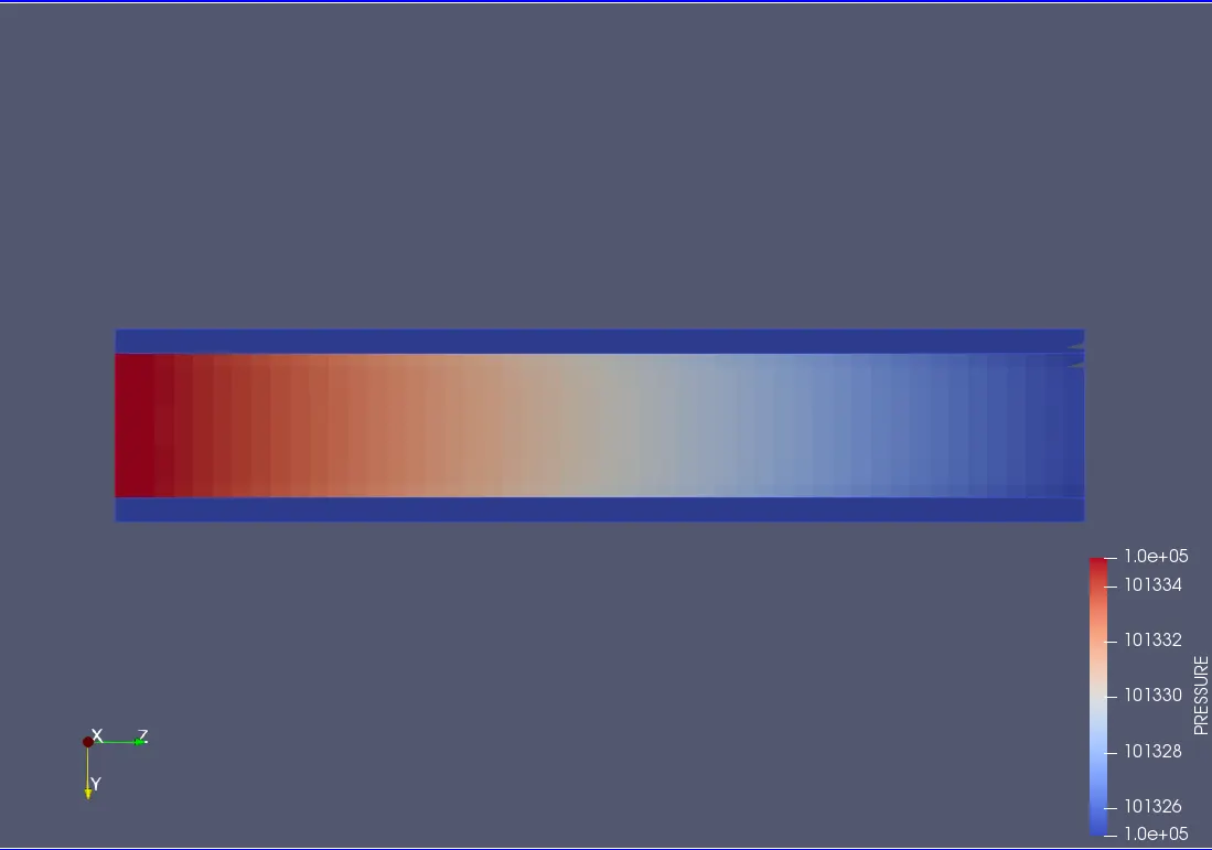
Pressure Contour:
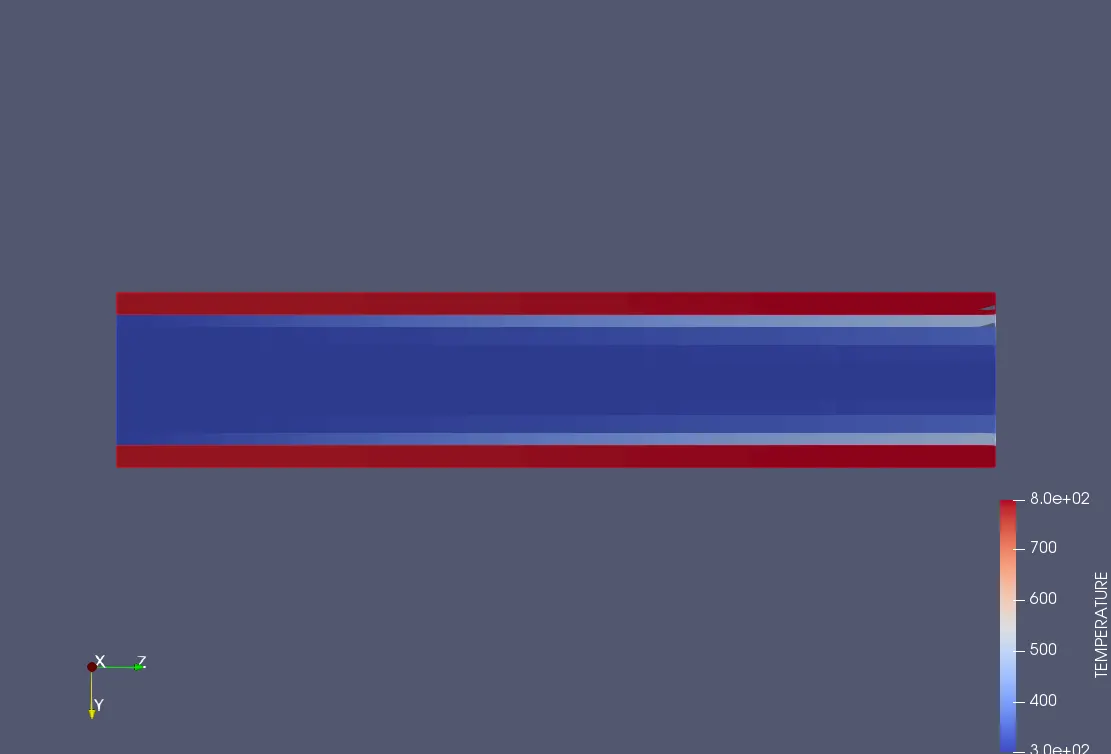
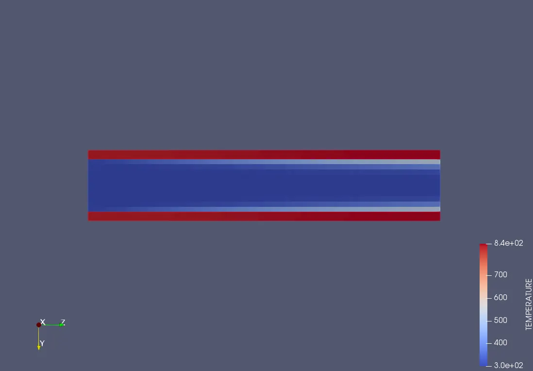
Temperatue Contour:
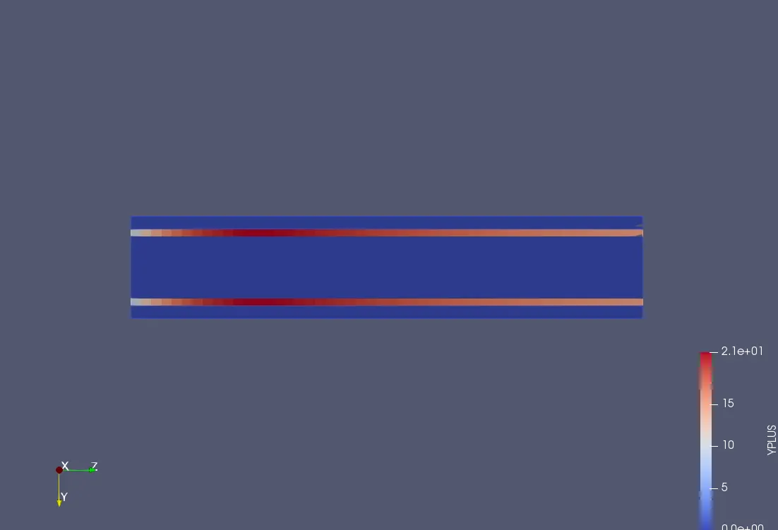
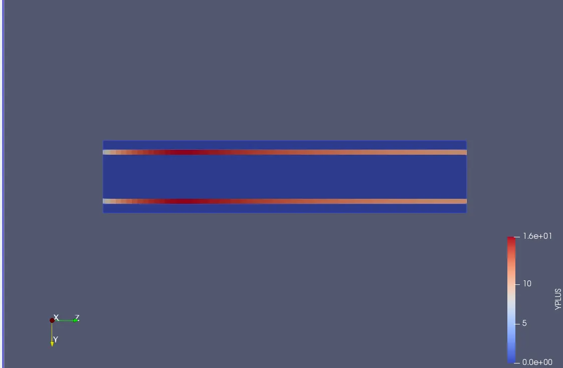
Y-Plus:
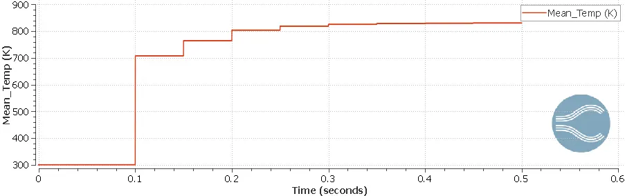
Temperature Plot:
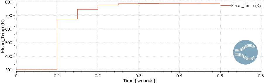
The Youtube link for the animation of velocity,temperature and pressure contours are given below,
Case Study 2: Mesh Size 0.003m :
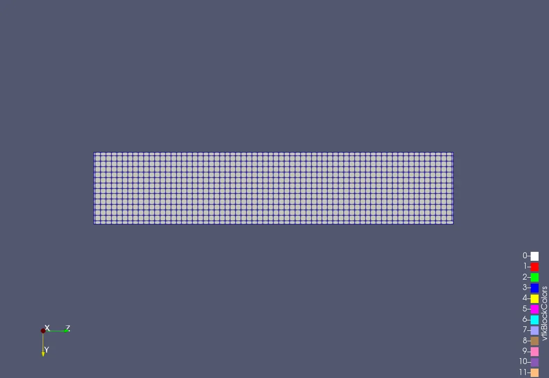
Generated Mesh:
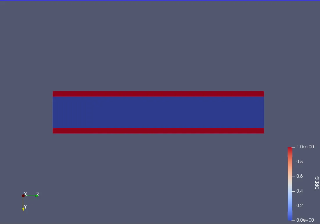
IDREG:
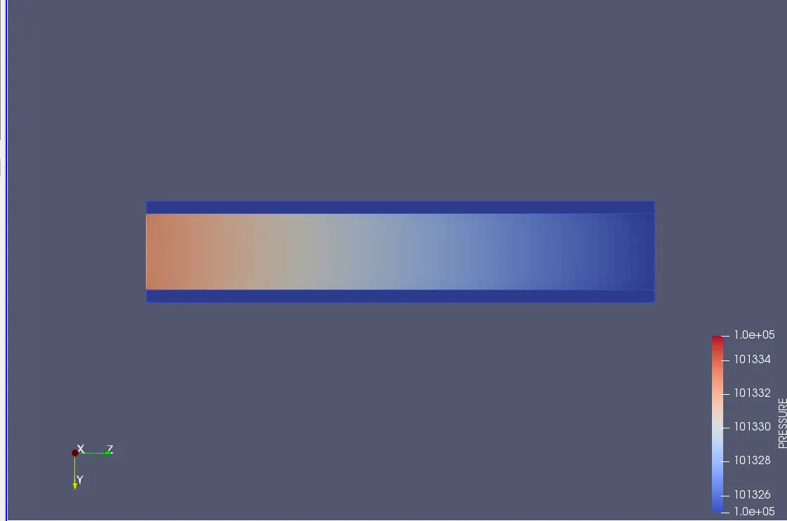
Pressure Contour:
Temperature Contour:
Velocity Contour:
Y-Plus:
Temperature Plot:
The Youtube link for the animation of velocity,temperature and pressure contours are given below,
Case Study 3: Mesh Size 0.003m :
Generated Mesh:
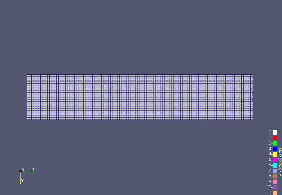
IDREG:
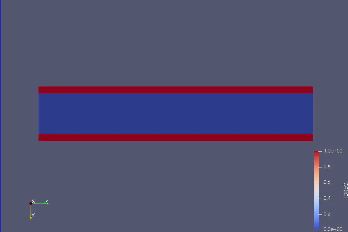
Pressure Contour:
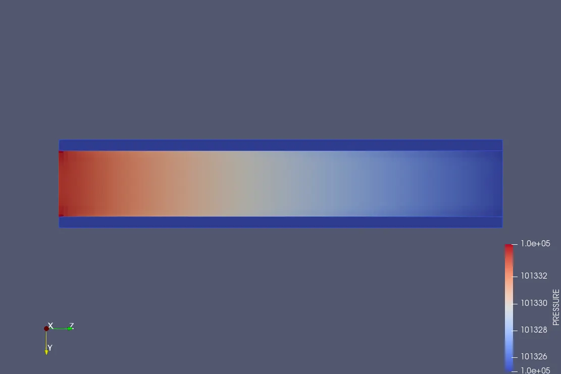
Temperature Contour:
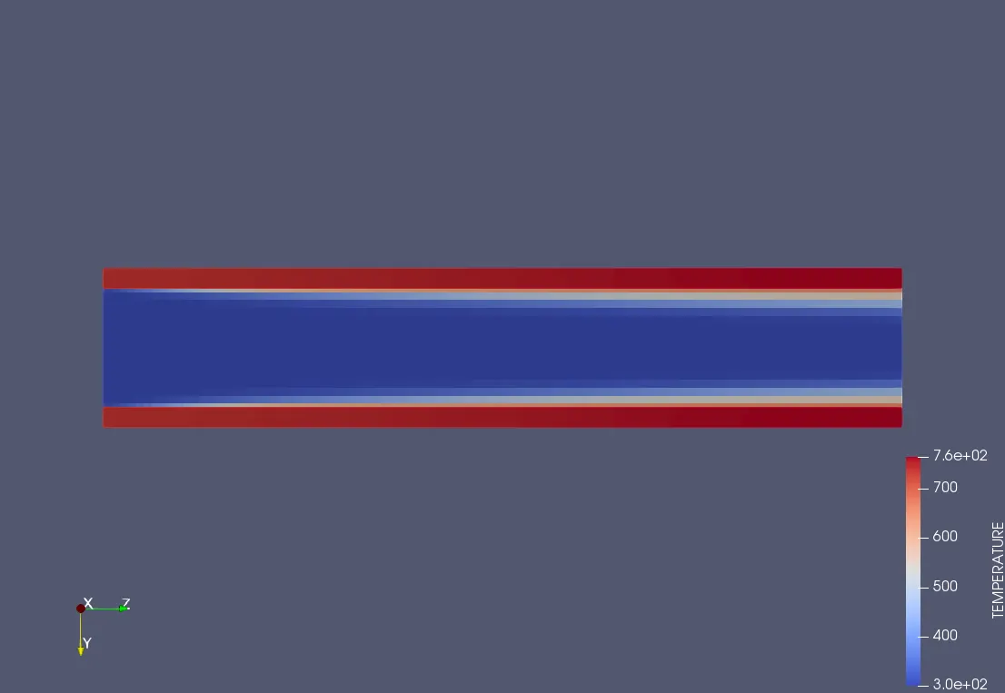
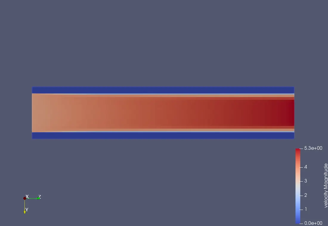
Velocity Contour:
Y-Plus:
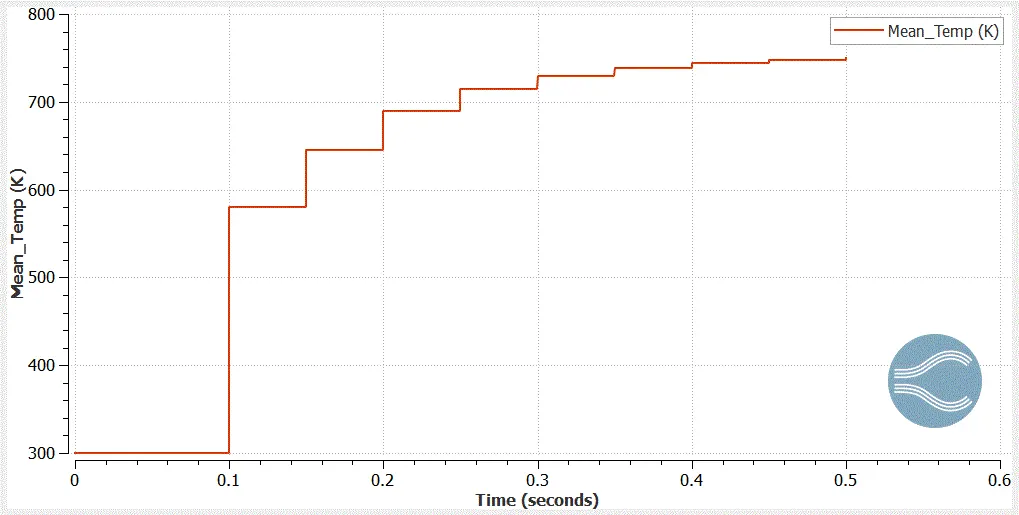
Temperature Plot:
The Youtube link for the animation of velocity,temperature and pressure contours are given below,