Mini project - Flow over an Airfoil

Aim

The major objective of this simulation was to set a simulation over the NACA 2412 aerofoil with different angles of attack(AOA) using Converge CFD and estimating its coefficient of lift and drag.

Introduction:

Airfoil is a structure that provides required Lift force and Drag force depending on profile design i.e. curved surface when an Airfoil structure moved in a fluid medium, it provides the aerodynamic forces. Therefore it is quite important to understand the importance behind the shape of Airfoil. As CFD is a powerful tool used to carry out the simulation by considering the real-life behavior of the fluid. In this study, the main objective is to carry out a detailed study on lift and drag coefficients of NACA2412 Airfoil sections with different AOA. Setting up the simulation in Converge CFD studio, solving it using Cygwin, and post-processing the contour plots using ParaView.

Angle Of Attack (AOA)

`1^circ`

`5^circ`

`10^o`

`15^o`

Aerofoil: Terminology and Definitions

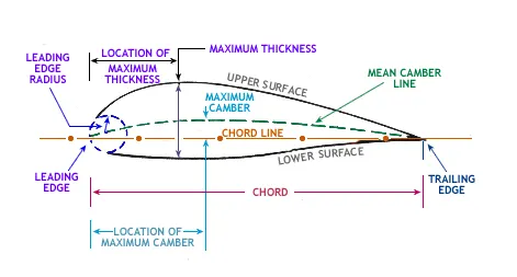
Aerofoil sketch is shown in Figure, which illustrates terminology:

1. Mean camber line- A line drawn halfway between the upper and lower surfaces of the aerofoil.

2. Leading-edge- It is the front edge of aerofoil where maximum curvature can be found.

3. Trailing edge- It is the rearmost edge of an aerofoil.

4. Chord line- It is the connecting line between leading and trailing edge and it is straight.

5. Chord length- It is the length of the chord line.

6. Camber- It is the maximum perpendicular distance between the mean camber line to chord line.

7. Thickness- It is measured either perpendicular to the camber line or perpendicular to the chord line.

8. The angle of attack- It is defined as the angle between the chord line and the relative wind or flight path.

Nomenclature of NACA-4 Digit Aerofoil

The NACA four-digit aerofoil sections define the profile by:

The first digit provides maximum camber which is in the percentage of the total chord length.

The second digit provides the distance of maximum camber from the leading edge in tens of percent of the total chord length.

The last two digits describe the maximum thickness of the aerofoil as a percentage of the total chord length.

For example, NACA 2415 aerofoil has a total chord length of 100 mm. So aerofoil has maximum camber 2mm which is 40mm far from leading edge with 15mm thickness.

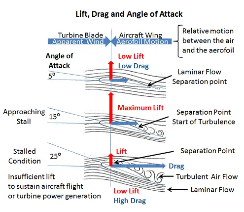
Lift coefficient (CL)- It is a dimensionless coefficient that relates the lifting force on the body to its velocity, surface area, and the density of the fluid in which it is lifting.

Lift force - It is a force that is perpendicular to the relative wind.

Lift Force=12⋅Cl⋅ρ⋅A⋅V2">Lift Force=`1/2*C_l*rho*A*V^2`

Drag coefficient (Cd)- It is a dimensionless coefficient that relates the dragging force on the body to its velocity, surface area, and the density of the fluid in which it is moving.

Drag force - It is a force that is parallel to the relative wind.

Drag Force=12⋅Cd⋅ρ⋅A⋅V2">Drag Force=`1/2*C_d*rho*A*V^2`

At very low angles of attack, the airflow over the aerofoil is essentially smooth and laminar with perhaps a small amount of turbulence occurring at the trailing edge of the aerofoil. The point at which laminar flow ceases and turbulence begins is known as the separation point.

Increasing the angle of attack increases the area of the aerofoil facing directly into the wind. This increases the lift but it also moves the separation point of laminar flow of the air above the aerofoil part way up towards the leading edge and the result of the increased turbulent flow above the aerofoil is an increase in the drag.

A maximum lift typically occurs when the angle of attack is around 15 degrees but this could be higher for specially designed aerofoils.

Above 15 degrees, the separation point moves right up to the leading edge of the aerofoil and laminar flow above the aerofoil is destroyed. The increased turbulence causes the rapid deterioration of the lift force while at the same time it dramatically increases the drag, resulting in a stall.

1.Geometry Creation

First of all, the Aerofoil geometry was setup using converge CFD software. The geometry was separately prepared using different CAD package ie Solidworks, then .stl file was imported to Converge Studio to set up the case study. The aerofoil coordinates were imported and then the "curve through the XYZ" feature was used in Solidworks for this geometry preparation.

http://airfoiltools.com/airfoil/naca4digit

For each case, the cord length was taken as 50mm, in order to run the simulation in less time because of shorter wind tunnel distance. A virtual wind Tunnel was setup using Solidworks.

Horizontal Length of Wind Tunnel is 50*The chord length

Vertical Length of Wind Tunnel is 30×The chord Length">30*the Chord length

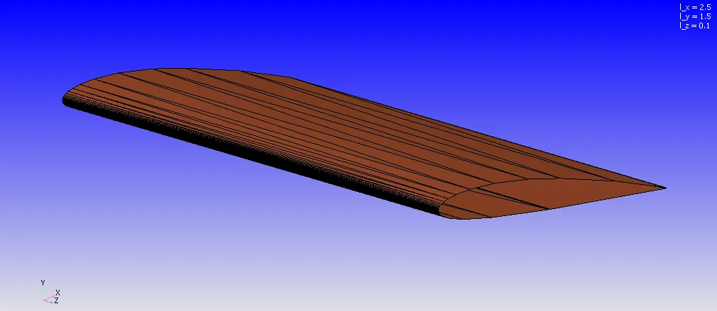
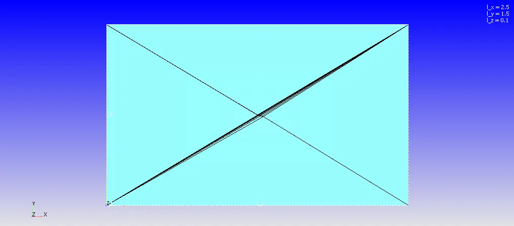
*Each face of the step was split into triangles.

The Box Dimension is :

Dx(m)	Dy(m)	Dz(m)
2.5	1.5	0.1

To create the geometry, the geometry was uploaded from the different CAD software package. All the normal vector were pointing out for this geometry, so we wanted it to point inside and normal to each surface. Normals point the direction of the fluid region generally. The command "Transform" was used to make the normal inside pointing the direction of the fluid region.

2.Boundary Creation

After creating the Aerofoil along with Wind Tunnel Geometry, The Boundry tag was created along with different boundary id and coloring. A total of 6 different boundaries tag was created for multiple different split triangles of the geometry with each face split into multiple triangles. To create the boundaries naming, the "Boundary" command in the "Geometry" dock was used, and then the faces were appointed to appropriate tags along with id.

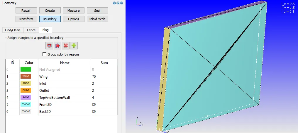
The six different boundaries were Inlet, Outlet, Top-Bottom, Front2D, Wing, and Back2D.

3.Case-Study Setup

The various parameter was considered while setup this case study. The case study setup dock was used to set up the problem which appears on the right-hand side of the converge studio.

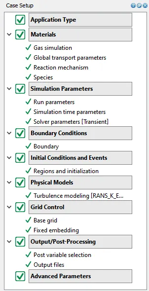
3.1 Application Type:

In order to run a steady-state simulation, firstly, under the Application type in the setup tree, a "Time-based" simulation must be selected.

3.2 Materials:

Under the material tab "Gas simulation" was selected and "Air" as a predefined mixture.

Gas: Air

Global Transport Parameters: Fixed value

by default, the following value is considered.

Prandtl Number : 0.9

Schmidt Number : 0.78

Species: Oxygen-O2 & Nitrogen-N2

Reaction Mechanism (mech.dat) was selected for this problem.

3.3 Simulation Parameters

The Transient solver was selected for running this case study along with a "Density-based" solver.

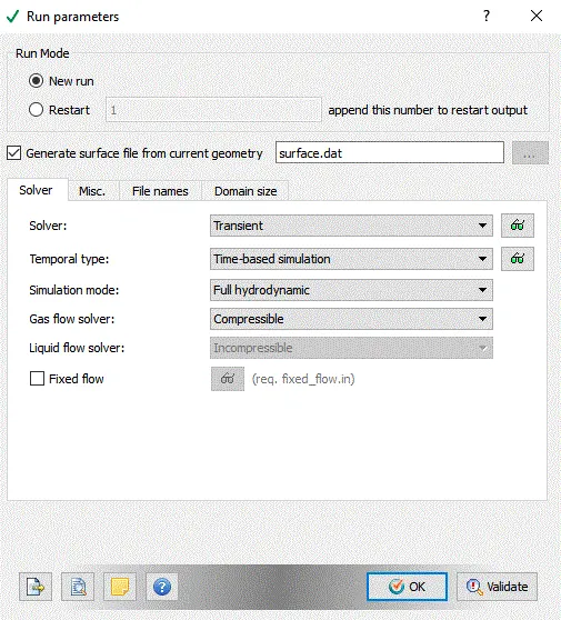
Calculation

Horizontal length=2.5m

Average Velocity=60.8m/s

Speed=Distance/time

therefore, Time=0.041 sec

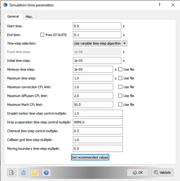
we are simulating roughly two times of flow through time that is 0.1s

The Following Simulation parameters were selected for running this simulation.

3.4: Boundary Conditions

In this tab, The volumetric region and physics for each boundary were defined.

Reynolds Number Re=200000

The density of Air(at 300k)=`rho=1.766(kg)/m^3`

Dynamic Viscosity(at 300k)=`mu=0.00001846(kg)/(ms)`

Kinematic Viscosity=`mu/rho=1.56893E-05(m^2)/s`

Characteristic length=50mm

Average Flow Velocity=`(Re*mu)/(rho*L)=60.8m/s`

Boundary_Name	Boundary_Type	Paramter_Defined	Boundary ID
1.Inlet	Inflow	60.8 m/s in X axis	2
2.Outlet	OutFlow	101325.0 Pa	3
3.Front2D	TWO_D		5
4.Back2D	TWO_D		6
5.TopAndBottomWall	Symmetry		4
6.Wings	Law of Wall	Law of Wall	1

3.5: Initial Conditions and Events

Volumetric Region was created in order to assign this to all the boundary tag.

Species:- O2 (0.23) & N2 (0.77)

Pressure :101325Pa

Temperature:300K

The velocity of 60.8m/s in X-axis

3.6: Physical Models

A turbulent model was selected out of so many models.

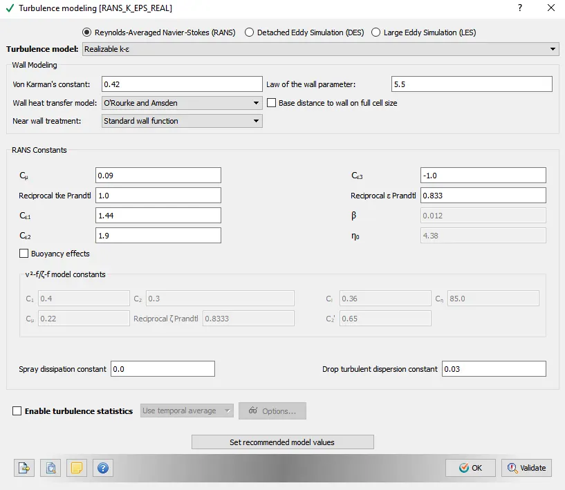
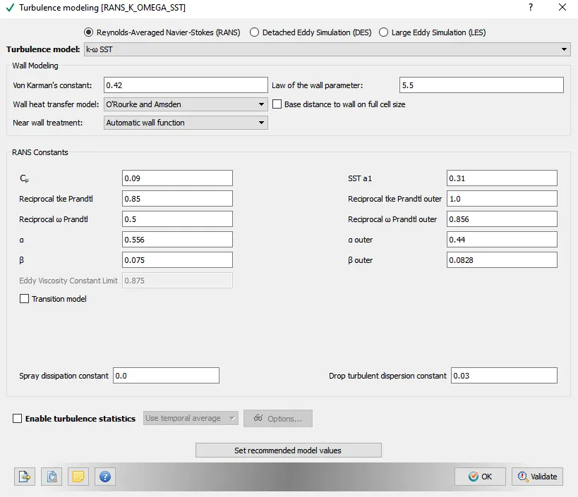
For the case study, 1 degree the Kω-SST">Kω−SST was selected and for 5 degrees, 10 degrees, 15 degrees Relizzible K-E">Relizzible K-E was selected.

3.7: Grid Control

The case study was run using a fine mesh grid size.

Base mesh sizes are,

S.No.	Dx(m)	Dy(m)	Dz(m)
1	0.004	0.004	0.004

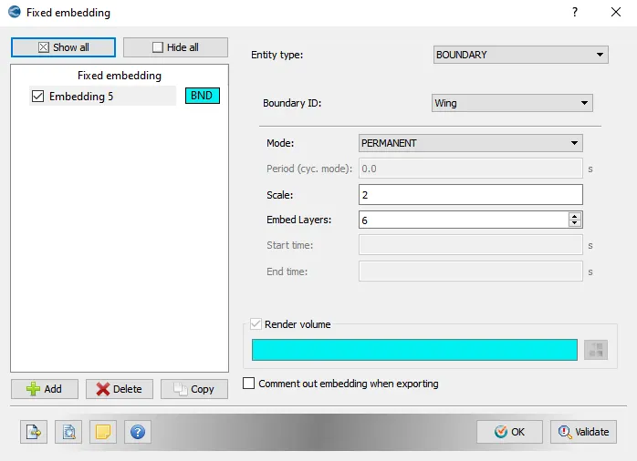
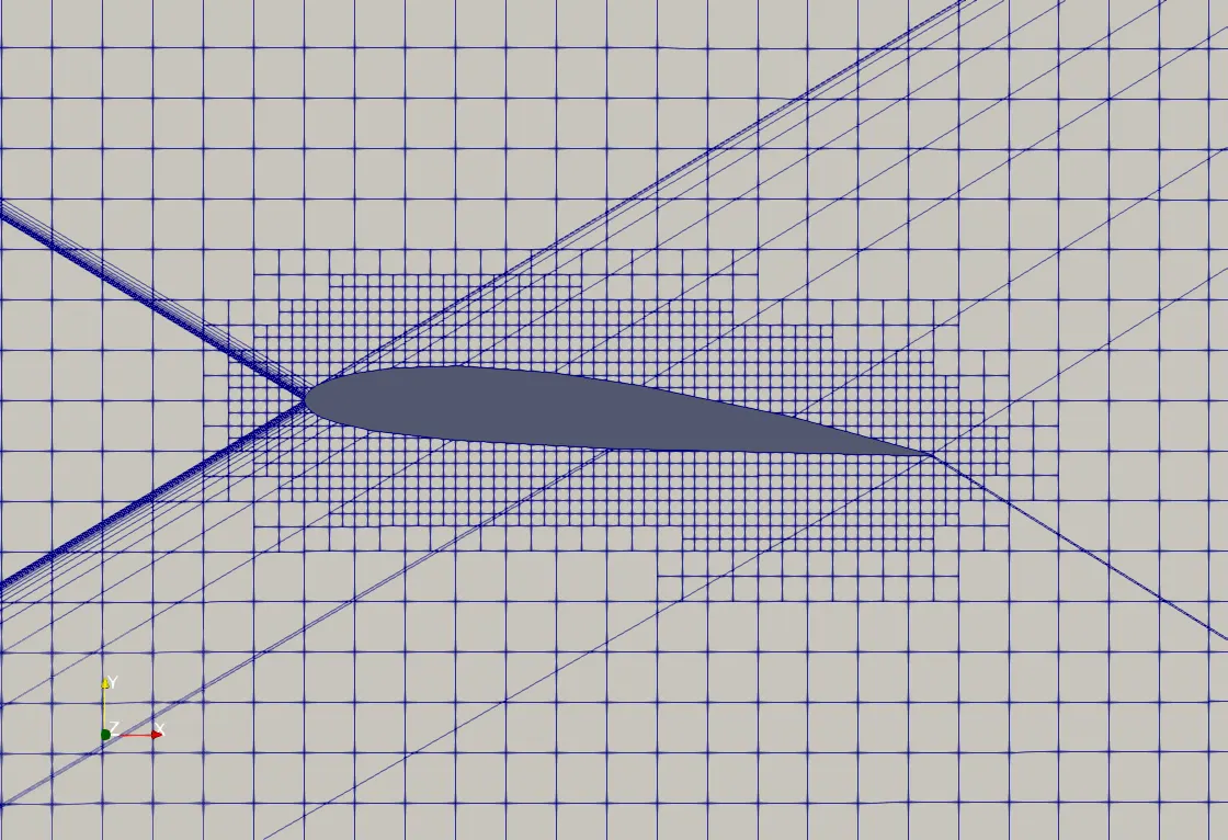
Fixed embedding was done in order to capture more cells near to aerofoil order to get more precise data.

Scale: 2 & Embed Layers: 6 near the wing

3.7 Output/Post-Processing

In regions and initialization, the value of velocity should be the same as that of Inlet velocity.

Also, while setting up the case, make sure, wall output (BOUNDARIES ONLY) is enabled as this will dump wall averaged output data which is very much important for any external aerodynamic simulations.

Post-Variable Selection- Existing value

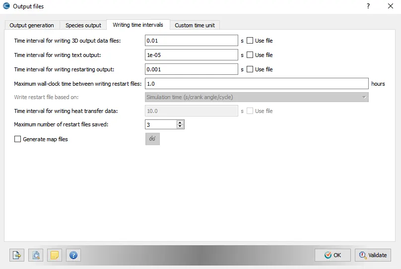
Output Files- Time interval for writing 3D output files-0.01 s

The time interval for writing restart files -0.001s

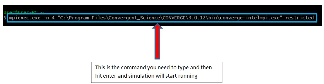
The case study was solved using CYGWIN and the post-processing was done in ParaView.

Simulation Result

Mesh

Case Study1: Angle of Attack 1 Degree

Velocity Contour

Velocity Contour

Pressure Contour

Pressure Contour

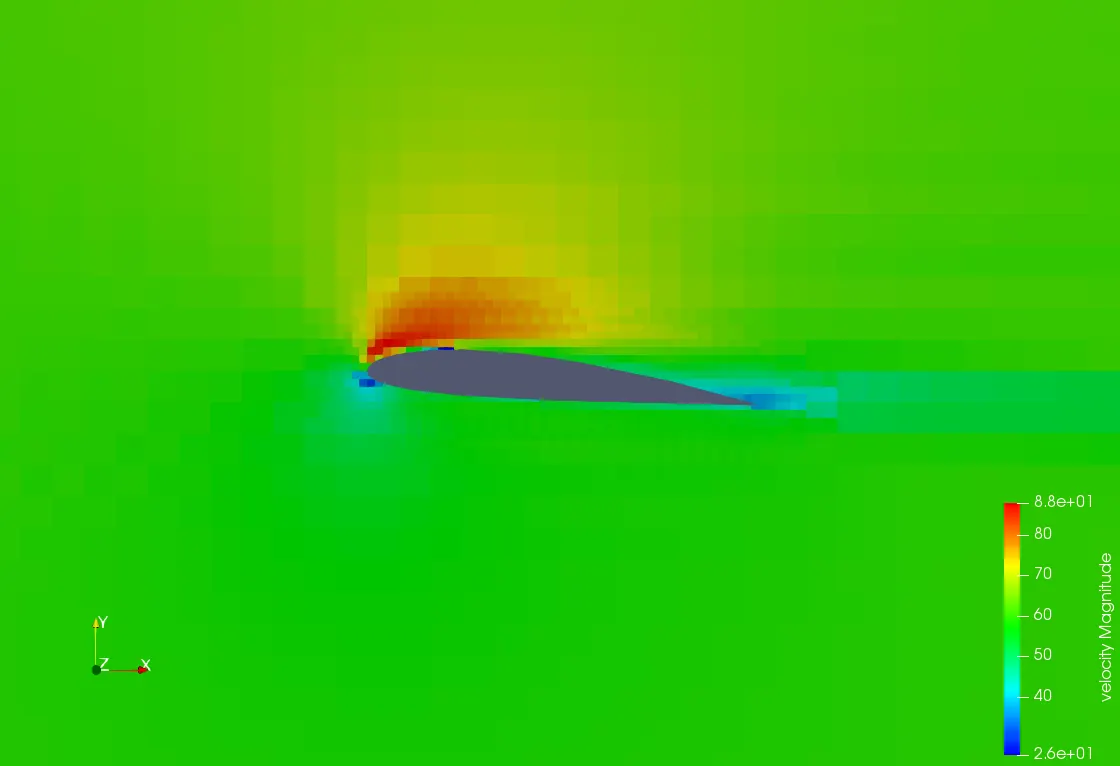
Case Study2: Angle of Attack 5 Degree

Velocity Contour

Velocity Contour

Pressure Contour

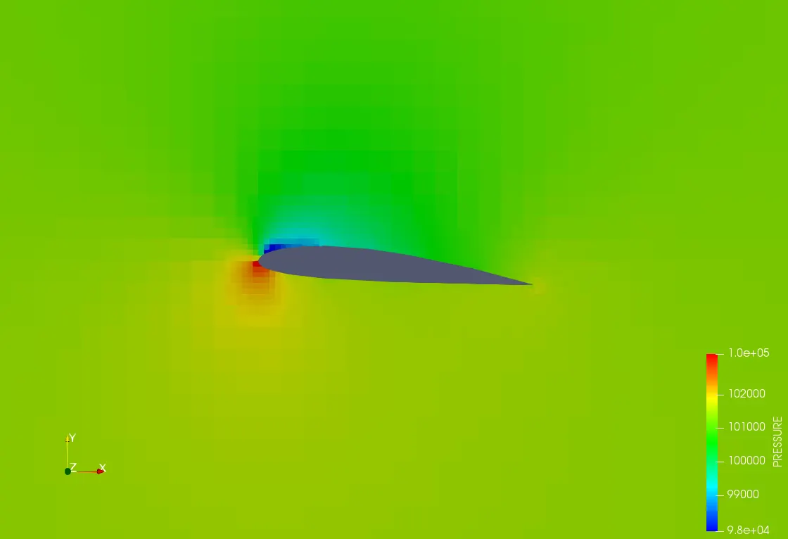
Pressure Contour

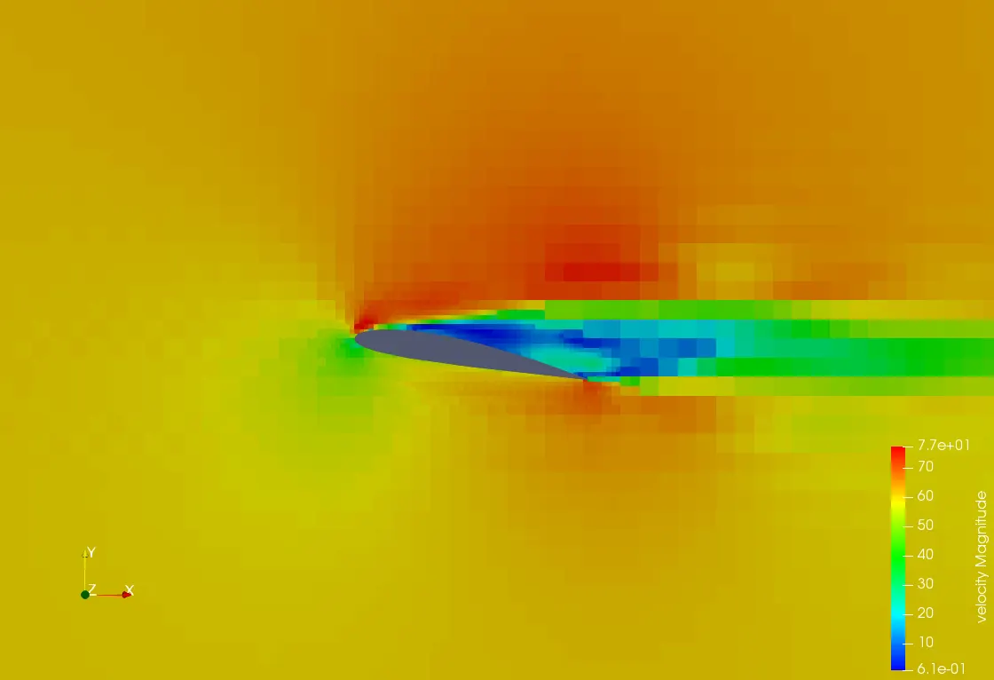
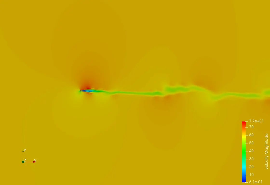
Case Study3: Angle of Attack 10 Degree

Velocity Contour

Velocity Contour

Pressure Contour

Pressure contour

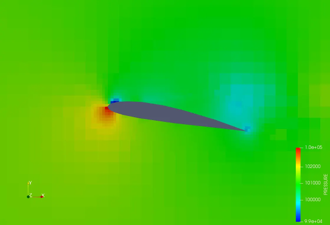
Case Study4: Angle of Attack 15 Degree

Velocity Contour

Velocity Contour

Pressure Contour

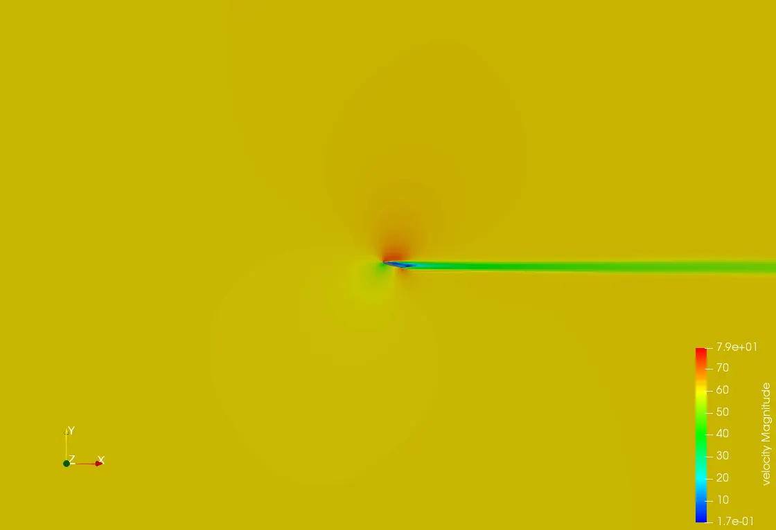
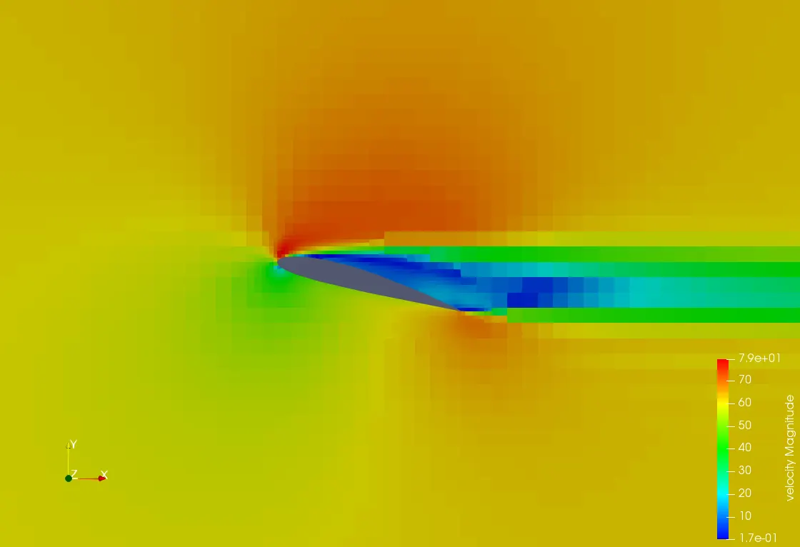
pressure Contour

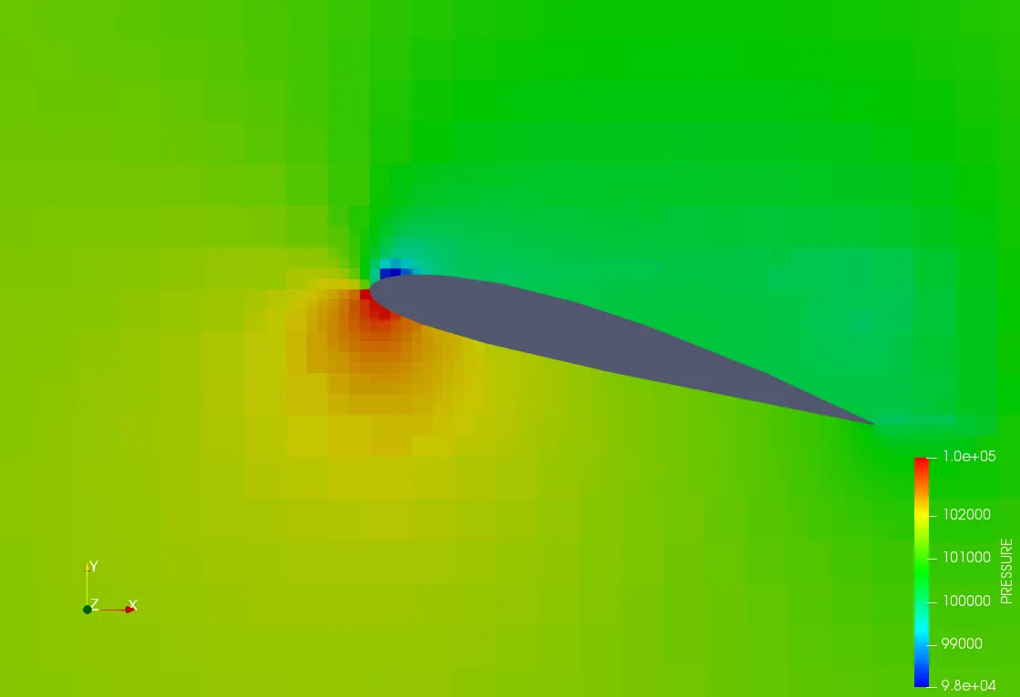
Line Plots

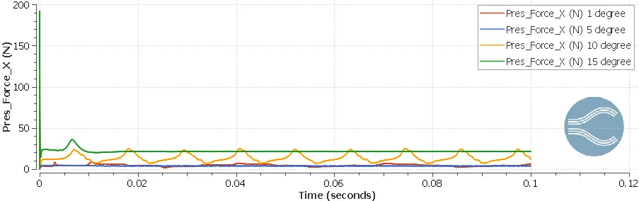
Drag Force

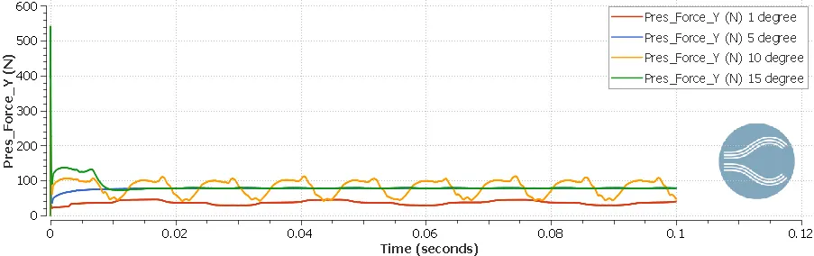
Lift Force

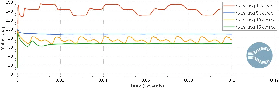
Y Plus

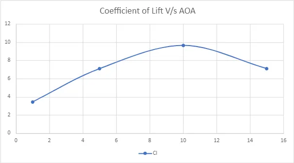
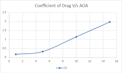
S.no.	Angle of Attack	Lift Force	Drag Force	Coefficient of Lift	Coefficient of Drag
1.	1 Deg	37.49 N	1.9N	3.44	0.174
2.	5 Deg	77.31 N	3.5N	7.1	0.321
3.	10 Deg	104.5 N	12.46N	9.66	1.146
4.	15 Deg	77.41 N	21.5N	7.11	1.977

Area=`0.05*0.1=0.005m^2`

Lift Force=`1/2*C_l*rho*A*V^2`

`C_l=(2L)/(rho*A*V^2)`

Drag Force=`1/2*C_d*rho*A*V^2`

`C_d=(2D)/(rho*A*V^2)`

Conclusion

AOA 1 Degree

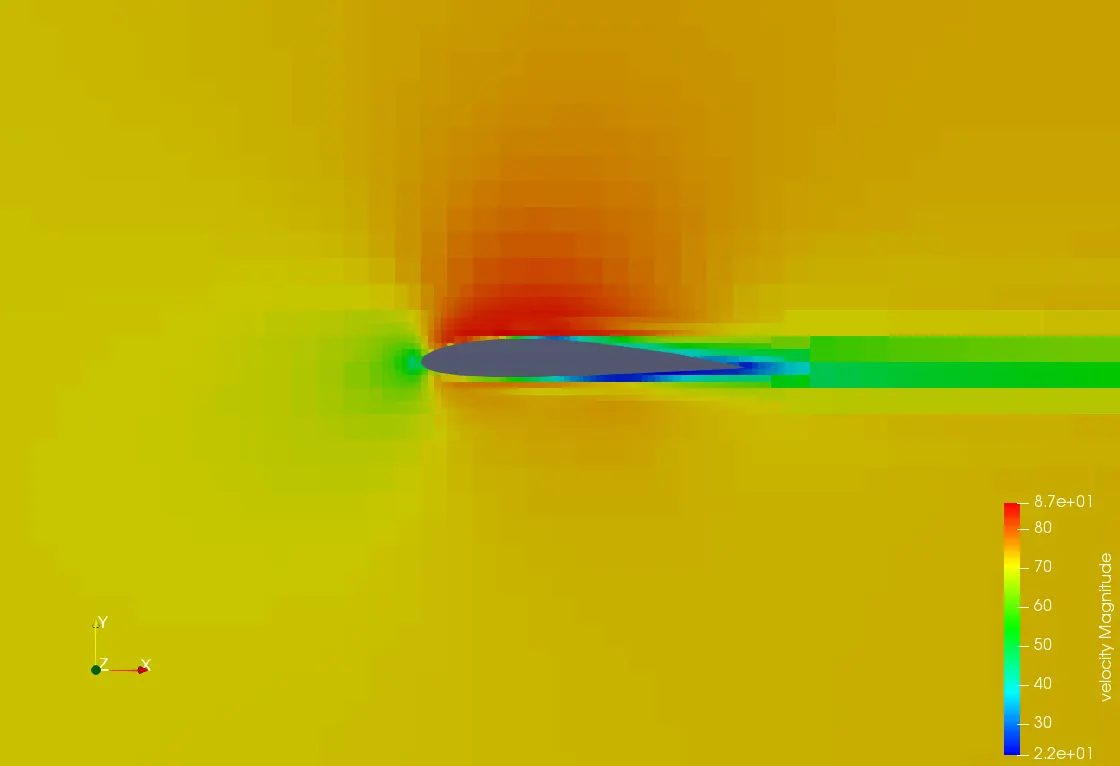
The velocity of air above the upper surface of the aero-foil is higher(indicated red) than that of the lower surface.
The velocity at the leading edge and the trailing edge are very low(indicated deep blue).

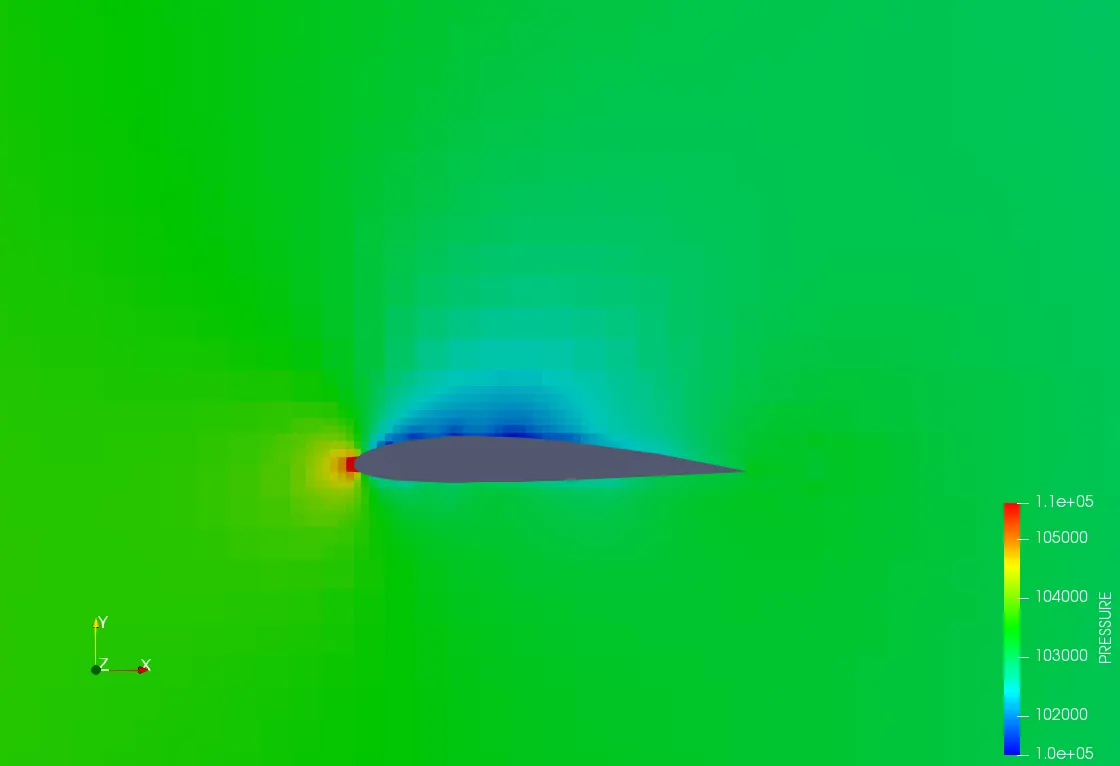
The pressure at the leading edge and the trailing edge is quite higher(indicated red).
The pressure of the air above the upper surface of the aero-foil is lower(indicated blue) than that of the lower surface.

Inference:
The velocity increases near the upper surface as the air gets diverted from its path and goes along with the stream of air actually upper surface. The velocity is very much lower at the leading edge as some amount of airstrikes the edge and loses its kinetic energy.
The velocity is little lesser in the trailing edge as a partial vacuum is created near it. This is accorded to the boundary layer formation in the aerofoil surface. Some amount of airstrikes the leading edge as it approaches the aero-foil, which causes an increase in pressure at this location. As the velocity is higher in the upper surface there is a pressure drop in this region, according to the less accumulation of fluid near the wing.

AOA 5 Degree

The pressure of air in the lower surface is far higher(indicated red) than that in the upper surface.
The pressure is very high at the leading edge(indicated deep red).

Inference:
As the airstrikes, the lower surface of the aero-foil, the kinetic energy of air is converted into pressure energy. Hence, as the airstrikes the pressure on the lower surface increases leading to positive pressure in the region. As the velocity is higher in the upper surface, the pressure is lower, leading to negative pressure. This combination of positive pressure on the lower surface and negative pressure on the upper surface leads to the production of lift. Some amount of airstrikes the leading edge as it approaches the aero-foil, which causes an increase in pressure at this location.

AOA 10and 15 Degree

Increasing the angle of attack increases the area of the aerofoil facing directly into the wind. This increases the lift but it also moves the separation point of laminar flow of the air above the aerofoil part way up towards the leading edge and the result of the increased turbulent flow above the aerofoil is an increase in the drag.

A maximum lift typically occurs when the angle of attack is around 10 degrees but this could be higher for specially designed aerofoils.

Above 15 degrees, the separation point moves right up to the leading edge of the aerofoil and laminar flow above the aerofoil is destroyed. The increased turbulence causes the rapid deterioration of the lift force while at the same time it dramatically increases the drag, resulting in a stall.

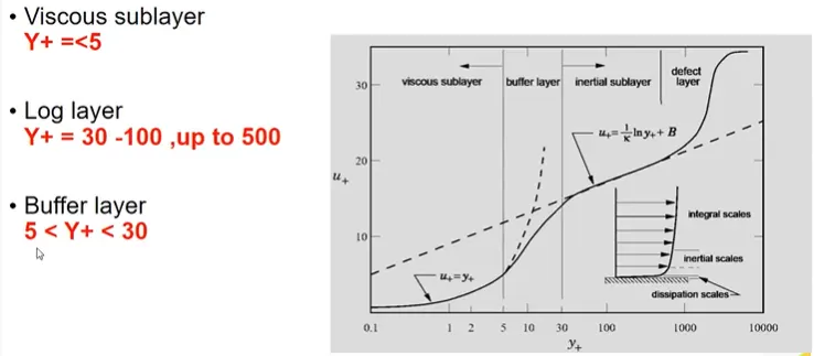
Turbulence is the state of chaotic and unstable fluid flow, just opposite of Laminar flow. Y plus(Y+) is the non-dimensional distance of the first cell from the wall.

Let's takes an example of a flat plate under zero pressure gradient and front left side the uniform velocity is coming to the plate. Firstly, it will be laminar flow, then after some disturbance, the region will be called as Transition Region, when the disturbance is growing too much the flow will change in Turbulent Flow. The boundary layer in the turbulent region will be called a turbulent boundary layer whereas in laminar it will be called the laminar boundary layer.

Reynold's Number ReRe is the ratio of Inertial force to the Viscous Force.

Viscous Sub Layer: Viscous stress term dominates

Buffer Layer: Transitional region

Log law Region: Reynolds shear stress term dominates

The Converge File can be downloaded from here Case setup