Simulation of Flow through a pipe in OpenFoam:

Objective :

To simulate the incompressible laminar flow through pipe using OpenFoam.

Things we need to do,

• Write a program in Matlab that can generate the computational mesh automatically for any wedge angle and grading schemes
  • Hint: wedge angle should be less than 5 degrees
  • Make sure that number of cells along the "axi symmetric"
• For a baseline mesh, show that the velocity profile matches with the Hagen poiseuille's equation
• Show that the velocity profile is fully developed
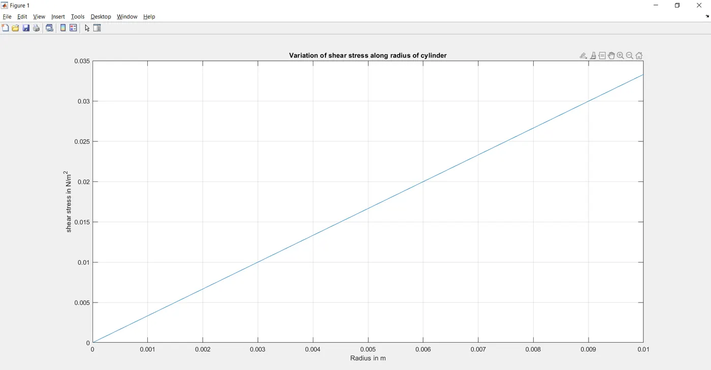
• Post process velocity and shear stress

Description :

Hagen poiseuille's equation - This is a physical law that gives the pressure drop in an incompressible and Newtonian fluid in laminar flow flowing through a long cylindrical pipe of constant cross section.

Length of the Enterance - The distance the fluid travels after entering a pipe before the complete development/ formation of the flow .

Hydrodynamic entrance region - Area of the pipe where the fluid entering a pipe developes a velocity profile due to the viscous forces that are spreading from the interior walls of pipes.

>> Here the fluid enters a pipe at a constant speed , hence fluid particles in the layer get contact with the pipe's surface come to a complete rest because of the non slip rule.

>> The layer taht is in contact with the pipe surface is resistant to the acceleration of the neighbouring layers due to the viscous forces produced within the fluid and gradually slows down the adjacent layers of the fluid, by forming a velocity profile.

>> To make the conservation of mass true, the velocity of the layers of the fluid at the center of the pipe increases in order to compensate the reduced velocities of the layer of fluid near the pipe surface.

>> Hence this generates a velocity gradient across the cross section of the pipe.

Fully developed region - Here the velocity profile does not change in the fluid flow direction.

Assumptions & considerations from Hagen Poiseuille equations :

Steps for solving the problem :

• Firstly in Linux OS open " Terminal ".
• Type ' cd $FOAM_TUTORIALS/ ', on typing this will direct to the inbuilt tutorial files in openFOAM software. Now to view the list of tutorials type ' ls '.
• Once the list opens, we can see multiple directories displayed. To select type ' cd incompressible/ '. As above to go into its list type ' ls '. Then it directs to the particular directory.
• As per the given data wee need to solve the flow using the icoFOAM solver. So type ' cd icoFOAM/ '. Go to the list and select cavity i.e. ' cd cavity/ '.
• Once we direct to the cavity folder it shows multiple files, here there is a file called ' cavity ' , this should be copied and paste the file to the ' run folder ' by using the command ' cp -r cavity $FOAM_RUN /(folder name where u saved the cavity in run folder without'/') '.
• Creating .txt file for blockMeshDict
• Initially, understanding the concept of Hagen poiseuilles's equation is important as several assumptions are made and neceessary formula's are used.
• Proper assumptions are made asa mentioned , so that we can have a better excution of program without any errors.
• From Hagen poiseuilles's equation calculate the equations so that we can check the solutions and list down all the formulaes that are required for the calculation, so that program runs smoothly.
• When we start the program, define all the assumptions that are made. Also include all the necessary equations that are to be calculated as shown in the program.
• Write a small code to calculate the shear stress vs radius of the pipe.
• Now to create a blockMeshDict file we using file parsing technique, reading and writing the files. These files are further used in our calculations or simulations as an input data.
• Firstly to create a header file follow the above steps manually or we can import the header part from the file existing and specify the line numbers so that it displays in correct sequence.
• In order to create a text file, use- '' f1 = fopen('blockMeshDict.txt','w') ". This command is used to write the data in the particular folder as mentioned.
• Follow the same sequence that is used in tutorial files and mention the necessary spacing as followed above. All the steps are covered in the programme.
• On completing the entry of all the neccessary data that is to be calculated for a blockMeshDict file, just type '' fclose(f1) ". This helps to close the text file.
• Hence this generates a ' .txt file ' as shown below. This file should be replaced with the existing file by removing .txt at the end of file name i.e. file name should only contain ' blockMeshDict '.
• Creating controlDict,transportProperties,u and p files
• Directly open the existing file of controlDict and change the values of start time, end time ,deltaT etc and save the file.
• Similarly, in transport Properties change the value of kinematic viscosity of the fluid as shown below and save the file.
• In the same way, make the necessary changes asper the inputs and considerations for u and p files and also save them.
• Go to the terminal and direct to the location where the files are saved and go to the cavity directory in run, by typing ' blockMesh '. By giving this command it structures the mesh and internal calculations are done for a perfect meshing. After the end of running theblockMesh, now check for the errors in the mesh by using ' checkMesh ' command.
• Hence if there are no errors after checking the mesh we can say that it is stable.
• Now use ' icoFoam ' command to run the simulation completely, this is because we used icoFoam as the solver for this problem. Wait untill it reaches the last time step. Check if it has excuited for all the time steps so that simulation goes smoothly. Also check if the courant number is less than 1.
• After the end of the simulation type ' paraFoam '. The command paraFoam directs to the paraview software directly by displaying the geometry.
• By using paraview software, geometry along with mesh is visualised and graphs are plotted as shown below.

Program in Matlab for creating a blockMeshDict file and showing variation of shear stress along radius of the cylinder :

(considering wedge angle =3degree)

clear all
close all
clc

%inputs
Re = 2100;  %Reynold Number.
D = 0.02;  %Dia of pipe in m.
rho = 997;  %Density of water in kg/m^3.
nu = 8.917e-7;  %Kinematic viscosity of water in m^2/s.

% Calculations
mu = rho*nu;  %Dynamic viscosity of water
%Re = rho*V_avg*D/mu;
V_avg = mu*Re/(rho*D);
V_max = 2*V_avg;

r = D/2;  %Radius of pipe in m.

L_entrance = 0.06*D*Re;  %Hydrodynamic length at the enterance.
L = L_entrance + 0.3;  %Total length of the pipe.

%Hagen Poiseulle equation
delta_p = 8*mu*V_avg*L/r^2;  %Pressure in Pa.
Kinematic_P = delta_p/rho;  %Kinematic Pressure in m^2/s^2.

%Wedge Angle
theta = input("Enter the value of the wedge angle:"); %wedge angle should be less than 5deg.

% calculacting shear stress
R = linspace(0,D/2,1000);


for i = 1:length(R)
    tau(i) = 2*mu*V_max*(abs(R(i)))/r^2;
end

%Plot
plot(R,tau);
xlabel('Radius in m');
ylabel('shear stress in N/m^2');
title('Variation of shear stress along radius of cylinder')
grid on
hold on


% creating blockMeshDict file:

%Calculating vartices
v0 = [0 0 0];
v1 = [0 r*cosd(theta/2) -r*sind(theta/2)];
v2 = [0 r*cosd(theta/2)  r*sind(theta/2)];
v3 = [L 0 0];
v4 = [L r*cosd(theta/2) -r*sind(theta/2)];
v5 = [L r*cosd(theta/2)  r*sind(theta/2)];

% Header file in openFoam
h1 ='/*--------------------------------*- C++ -*----------------------------------*';
h2 ='| =========                 |                                                 |';
h3 ='| \      /  F ield         | OpenFOAM: The Open Source CFD Toolbox           |';
h4 ='|  \    /   O peration     | Website:  https://openfoam.org                  |';
h5 ='|   \  /    A nd           | Version:  8                                     |';
h6 ='|    \/     M anipulation  |                                                 |';
h7 ='*---------------------------------------------------------------------------*/';
h8 ='FoamFile';
h9 ='{';
h10 =  'version     2.0;';
h11 =  'format      ascii;';
h12=   'class       dictionary;';
h13 =  'object      blockMeshDict;';
h14 ='}';
h15 ='// * * * * * * * * * * * * * * * * * * * * * * * * * * * * * * * * * * * * * //';

f1 = fopen('blockMeshDict.txt','w');  % creating a text file.
fprintf(f1,'%s n',h1);
fprintf(f1,'%s n',h2);
fprintf(f1,'%s n',h3);
fprintf(f1,'%s n',h4);
fprintf(f1,'%s n',h5);
fprintf(f1,'%s n',h6);
fprintf(f1,'%s n',h7);
fprintf(f1,'n');
fprintf(f1,'%s n',h8);
fprintf(f1,'n');
fprintf(f1,'%s n',h9);
fprintf(f1,'%s n',h10);
fprintf(f1,'%s n',h11);
fprintf(f1,'%s n',h12);
fprintf(f1,'%s n',h13);
fprintf(f1,'%s n',h14);
fprintf(f1,'%s n',h15);
fprintf(f1,'n');

fprintf(f1,'%s n','convertToMeters 1;')
fprintf(f1,'n')

%Vertices
fprintf(f1,'%s n','vertices')
fprintf(f1,'%s n','(')
fprintf(f1,'t(%d %d %d)n',v0(1),v0(2),v0(3))
fprintf(f1,'t(%d %d %d)n',v1(1),v1(2),v1(3))
fprintf(f1,'t(%d %d %d)n',v2(1),v2(2),v2(3))
fprintf(f1,'t(%d %d %d)n',v3(1),v3(2),v3(3))
fprintf(f1,'t(%d %d %d)n',v4(1),v4(2),v4(3))
fprintf(f1,'t(%d %d %d)n',v5(1),v5(2),v5(3))
fprintf(f1,'%s n',');')

%blocks
fprintf(f1,'n')
fprintf(f1,'%s n','blocks')
fprintf(f1,'%s n','(')
fprintf(f1,'t hex (0 3 4 1 0 3 5 2) (%d %d %d) simpleGrading (1 0.1 1)n',300,30,1)
fprintf(f1,'%s n',');')

%edges
fprintf(f1,'n')
fprintf(f1,'%s n','edges')
fprintf(f1,'%s n','(')
fprintf(f1,'t arc 1 2 (%d %d %d)n',0,r,0)
fprintf(f1,'t arc 4 5 (%d %d %d)n',L,r,0)
fprintf(f1,'%s n',');')

%boundary
fprintf(f1,'n')
fprintf(f1,'%s n','boundary')
fprintf(f1,'%s n','(')
%axis
fprintf(f1,'t axis n t {n')
fprintf(f1,'t type empty;n')
fprintf(f1,'t faces nt ( n')
fprintf(f1,'t (%d %d %d %d)n',0,3,3,0)
fprintf (f1,'tt);n t}n')

%wall
fprintf(f1,'n')
fprintf(f1,'t wall n t {n')
fprintf(f1,'t type wall;n')
fprintf(f1,'t faces n t(n')
fprintf(f1,'t (%d %d %d %d)n',1,4,5,2)
fprintf(f1,'tt);n t}n')

%inlet
fprintf(f1,'n')
fprintf(f1,'t inlet n t {n')
fprintf(f1,'t type patch;n')
fprintf(f1,'t faces nt ( n')
fprintf(f1,'t (%d %d %d %d)n',0,1,2,0)
fprintf (f1,'tt);n t}n')

%outlet
fprintf(f1,'n')
fprintf(f1,'t outlet n t {n')
fprintf(f1,'t type patch;n')
fprintf(f1,'t faces nt ( n')
fprintf(f1,'t (%d %d %d %d)n',3,5,4,3)
fprintf (f1,'tt);n t}n')

%front
fprintf(f1,'n')
fprintf(f1,'t front n t {n')
fprintf(f1,'t type wedge;n')
fprintf(f1,'t faces nt ( n')
fprintf(f1,'t (%d %d %d %d)n',0,3,4,1)
fprintf (f1,'tt);n t}n')

%back
fprintf(f1,'n')
fprintf(f1,'t back n t {n')
fprintf(f1,'t type wedge;n')
fprintf(f1,'t faces nt ( n')
fprintf(f1,'t (%d %d %d %d)n',0,2,5,3)
fprintf (f1,'tt );n t}n tt );n')

fprintf(f1,'n')

fprintf(f1, '%s n','mergePatchPairs')
fprintf(f1,'t(n tt ); n')

fprintf(f1,'// ************************************************************************* //')
fclose(f1)

blockMeshDict file:

/*--------------------------------*- C++ -*----------------------------------*\
  =========                 |
  \\      /  F ield         | OpenFOAM: The Open Source CFD Toolbox
   \\    /   O peration     | Website:  https://openfoam.org
    \\  /    A nd           | Version:  8
     \\/     M anipulation  |
\*---------------------------------------------------------------------------*/
FoamFile
{
    version     2.0;
    format      ascii;
    class       dictionary;
    object      blockMeshDict;
}
// * * * * * * * * * * * * * * * * * * * * * * * * * * * * * * * * * * * * * //

convertToMeters 1; 

vertices 
( 
	(0 0 0)
	(0 9.996573e-03 -2.617695e-04)
	(0 9.996573e-03 2.617695e-04)
	(2.820000e+00 0 0)
	(2.820000e+00 9.996573e-03 -2.617695e-04)
	(2.820000e+00 9.996573e-03 2.617695e-04)
); 

blocks 
( 
	 hex (0 3 4 1 0 3 5 2) (300 30 1) simpleGrading (1 0.1 1)
); 

edges 
( 
	 arc 1 2 (0 1.000000e-02 0)
	 arc 4 5 (2.820000e+00 1.000000e-02 0)
); 

boundary 
( 
   axis 
   {
      type empty;
      faces 
      ( 
         (0 3 3 0)
      );
   }
   wall 
   {
      type wall;
      faces 
      (
         (1 4 5 2)
      );
   }

   inlet 
   {
      type patch;
      faces 
      ( 
         (0 1 2 0)
      );
   }

   outlet 
   {
      type patch;
      faces 
      ( 
         (3 5 4 3)
      );
   }

   front 
   {
      type wedge;
      faces 
      ( 
         (0 3 4 1)
      );
   }

   back 
   {
      type wedge;
      faces 
      ( 
         (0 2 5 3)
      );
   }
);

mergePatchPairs 
(
 		
); 
// ************************************************************************* //

controlDict file :

/*--------------------------------*- C++ -*----------------------------------*
  =========                 |
  \      /  F ield         | OpenFOAM: The Open Source CFD Toolbox
   \    /   O peration     | Website:  https://openfoam.org
    \  /    A nd           | Version:  8
     \/     M anipulation  |
*---------------------------------------------------------------------------*/
FoamFile
{
    version     2.0;
    format      ascii;
    class       dictionary;
    location    "system";
    object      controlDict;
}
// * * * * * * * * * * * * * * * * * * * * * * * * * * * * * * * * * * * * * //

application     icoFoam;

startFrom       startTime;

startTime       0;

stopAt          endTime;

endTime         10;

deltaT          1e-3;

writeControl    timeStep;

writeInterval   100;

purgeWrite      0;

writeFormat     ascii;

writePrecision  6;

writeCompression off;

timeFormat      general;

timePrecision   6;

runTimeModifiable true;


// ************************************************************************* //

transport Properties file:

/*--------------------------------*- C++ -*----------------------------------*
  =========                 |
  \      /  F ield         | OpenFOAM: The Open Source CFD Toolbox
   \    /   O peration     | Website:  https://openfoam.org
    \  /    A nd           | Version:  8
     \/     M anipulation  |
*---------------------------------------------------------------------------*/
FoamFile
{
    version     2.0;
    format      ascii;
    class       dictionary;
    location    "constant";
    object      transportProperties;
}
// * * * * * * * * * * * * * * * * * * * * * * * * * * * * * * * * * * * * * //

nu              [0 2 -1 0 0 0 0] 8.917e-7;


// ************************************************************************* //

velocity (U) file:

/*--------------------------------*- C++ -*----------------------------------*
  =========                 |
  \      /  F ield         | OpenFOAM: The Open Source CFD Toolbox
   \    /   O peration     | Website:  https://openfoam.org
    \  /    A nd           | Version:  8
     \/     M anipulation  |
*---------------------------------------------------------------------------*/
FoamFile
{
    version     2.0;
    format      ascii;
    class       volVectorField;
    object      U;
}
// * * * * * * * * * * * * * * * * * * * * * * * * * * * * * * * * * * * * * //

dimensions      [0 1 -1 0 0 0 0];

internalField   uniform (0.09363 0 0);

boundaryField
{
    axis
    {
        type            empty;
    }
    
    wall
    {
        type            noSlip;
    }
    
    inlet
    {
        type            fixedValue;
        value           uniform (0.09363 0 0);
    }

    outlet
    {
        type            zeroGradient;
    }
    
    front
    {
        type            wedge;
    }
   
    back
    {
        type            wedge;
    }
}

// ************************************************************************* //

pressure (p) file:

/*--------------------------------*- C++ -*----------------------------------*
  =========                 |
  \      /  F ield         | OpenFOAM: The Open Source CFD Toolbox
   \    /   O peration     | Website:  https://openfoam.org
    \  /    A nd           | Version:  8
     \/     M anipulation  |
*---------------------------------------------------------------------------*/
FoamFile
{
    version     2.0;
    format      ascii;
    class       volScalarField;
    object      p;
}
// * * * * * * * * * * * * * * * * * * * * * * * * * * * * * * * * * * * * * //

dimensions      [0 2 -2 0 0 0 0];

internalField   uniform 0;

boundaryField
{
    axis
    {
        type            empty;
    }
    
    wall
    {
        type            zeroGradient;
    }
    
    inlet
    {
        type            zeroGradient;
    }

    outlet
    {
        type            zeroGradient;
        value           uniform 0.018;
    }
    
    front
    {
        type            wedge;
    }
   
    back
    {
        type            wedge;
    }
}

// ************************************************************************* //
 

Post processing/ Results :

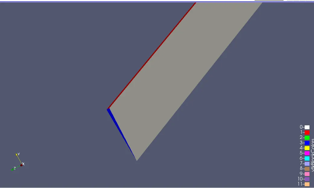
Geometry of wedge:

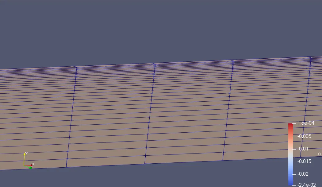
Generated Mesh:

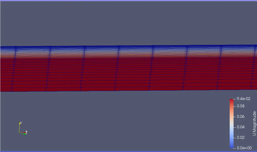
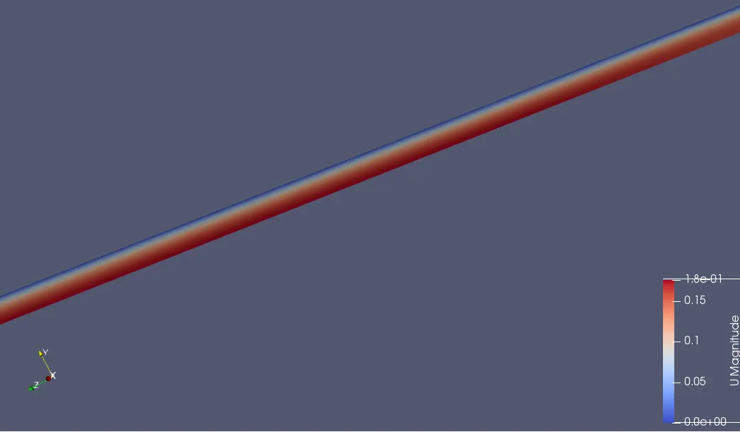
Generated velocity profile:

Generated plots : -

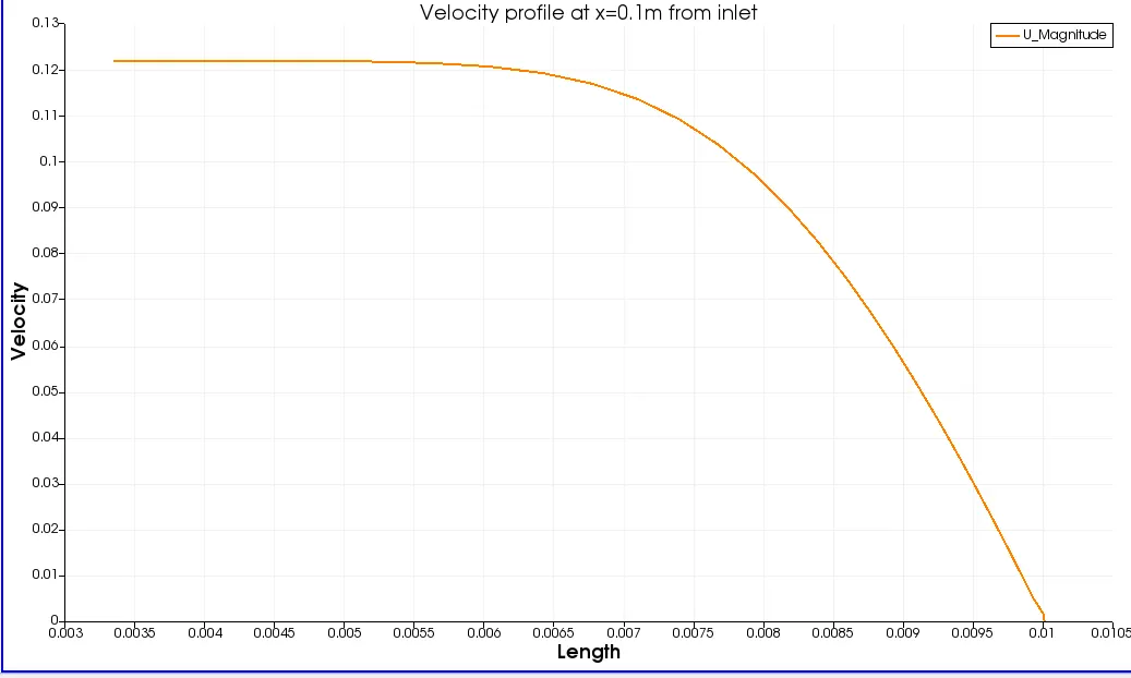
Velocity profile at 0.1m from inlet:

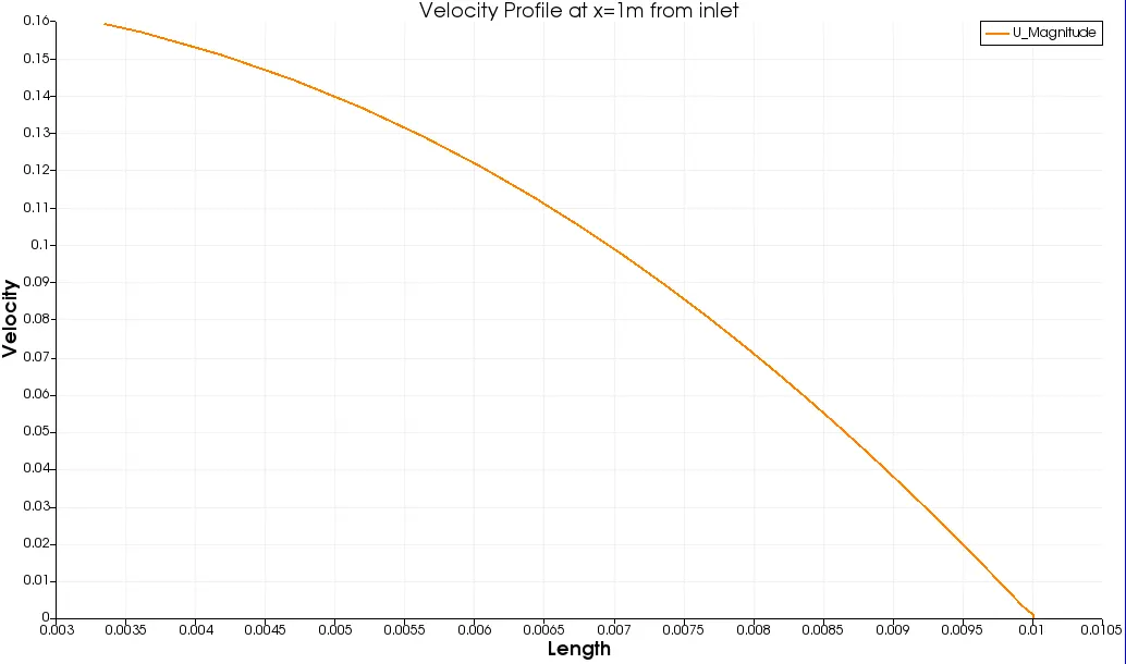
Velocity profile at 1m from inlet:

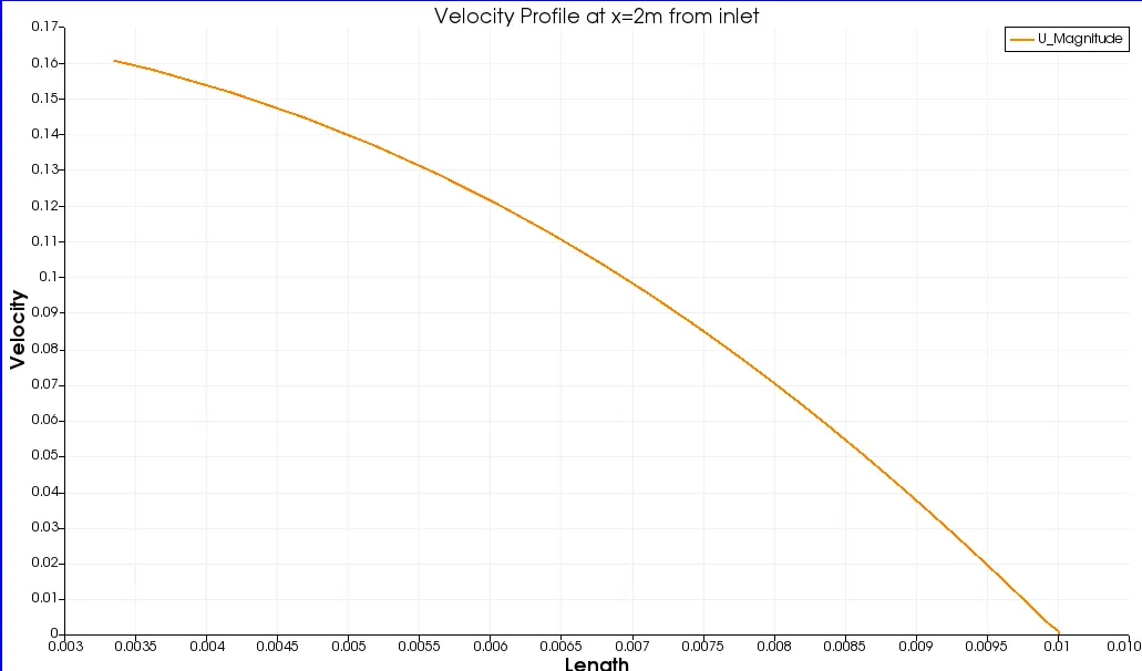
Velocity profile at 2m from inlet:

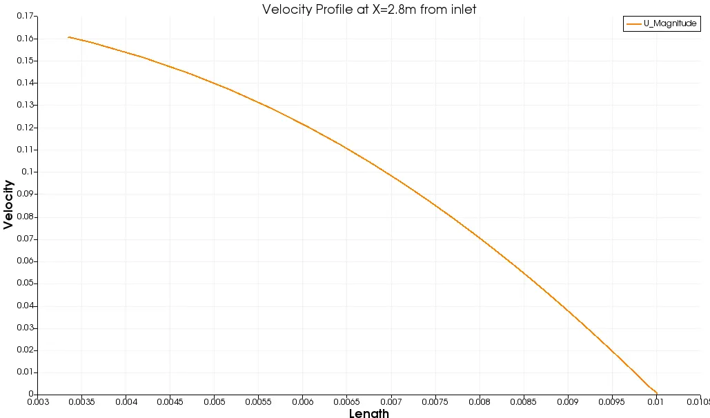
Velocity profile at 2.8m from inlet:

Shear stress profile:

>> Generally shear stress in laminar flow is a result of momentum transfer among the randomly moving molecules in a flow.

>> Analytically shear stress can be represented by the formulae -

Program to calculate the shear stress:

clear all
close all
clc

%inputs
Re = 2100;  %Reynold Number.
D = 0.02;  %Dia of pipe in m.
rho = 997;  %Density of water in kg/m^3.
nu = 8.917e-7;  %Kinematic viscosity of water in m^2/s.

% Calculations
mu = rho*nu;  %Dynamic viscosity of water
%Re = rho*V_avg*D/mu;
V_avg = mu*Re/(rho*D);
V_max = 2*V_avg;

r = D/2;  %Radius of pipe in m.

L_entrance = 0.06*D*Re;  %Hydrodynamic length at the enterance.
L = L_entrance + 0.3;  %Total length of the pipe.

%Hagen Poiseulle equation
delta_p = 8*mu*V_avg*L/r^2;  %Pressure in Pa.
Kinematic_P = delta_p/rho;  %Kinematic Pressure in m^2/s^2.

%Wedge Angle
theta = input("Enter the value of the wedge angle:"); %wedge angle should be less than 5deg.

% calculacting shear stress
R = linspace(0,D/2,1000);


for i = 1:length(R)
    tau(i) = 2*mu*V_max*(abs(R(i)))/r^2;
end

%Plot
plot(R,tau);
xlabel('Radius in m');
ylabel('shear stress in N/m^2');
title('Variation of shear stress along radius of cylinder')
grid on

Result:

Conclusions:

>> From all the above plots it is observed that the velocity profile gradually increased from inlet to the outlet i.e. (from x=0.1m to x=2.8m from the inlet). The velocity profile is observed to increase slowly at different lengths of pipe and also it reached maximum velocity at the outlet. This region is called as a fully developed region as the velocity profile completely developes at the outlet.

>> At the walls the velocity remains zero as we considered no slip boundary conditions. As the flowflow progress-gradually the boundary layers developand the adjacent layers tend to slow down. Because of this the velocity at the center increases. Hence, because of the pressure difference obtained from the equations, the velocity profile obayes Hagen Poiseuille's equation. Hence velocity profile matches with the Hagen poiseuille's equation.

>> When the fluid is moving, shear stresses are developed as the particles in the flow move relative to each other. For a fluif flowing in a pipe, the fluid velocity remains zero at the pipe wall. Shear force is generated because of the adjacent layer of the fluid that move with different velocities.

>> If value of mu is constant, the shear stress is linearly dependent on the velocity gradient. As the change in velocity is larger , more the shear stress near the walls.

>> Hence, the the computational mesh is generated for wedge angle =3degree. Also showed that the velocity profile matches the Hagen poiseuille's equation. From the above plotted velocity profiles it is proved that the profile is fully developed.