Modeling and Simulation of flow around an Ahmed Body:

Aim:

The major objective of this project was to model and set up the simulation of flow around an Ahmed Body using Converge CFD and Comparing the simulation result with the experimental data provided.

Introduction:

The Ahmed body is a generic car body (a simplified vehicle model). The airflow around the Ahmed body captures the essential flow features around an automobile and was first defined and characterized in the experimental work of Ahmed. Although it has a very simple shape, the Ahmed body allows us to capture characteristic features that are relevant to bodies in the automobile industry.

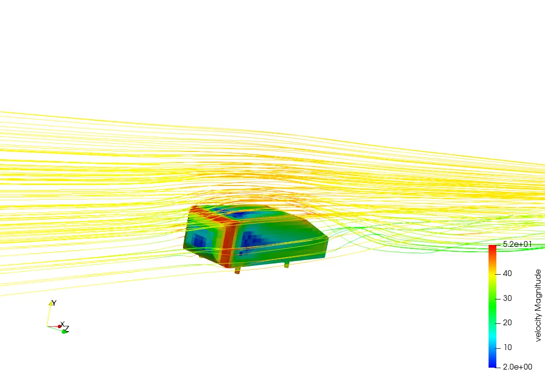
"The Ahmed reference model was originally developed for a time-averaged vehicle wake investigation (Ahmed et al. 1984). It is a car-like bluff body with a curved forebody, straight center section, and an angled rear end, representing a highly simplified ¼ scale lower medium-size hatchback vehicle. The specific angle of the back end can be altered between 0°and 40°. The model's major dimensions are 1044mm x 389mm x 288mm."

Boundary layer thickness is 30mm at 400mm in front of Ahmed body

`delta=(0.382*x)/(Re^2)`

Where `delta` is the boundary layer thickness in m which is 30m

"x" is the length of Plate(m).

`Re` is the Reynolds number.

`0.03=(0.382*x)/((rho*V*x^2)/mu)`

`x^0.8=0.03*((1.225*40)/(1.85*10^-5))/(0.382)`

`x=1.66m`

This means that 1.66m in front as the Ahmed body there will be boundary layer which is of 30mm thick.

So the Actual no-slip region in front of Ahmed body should be 1.66+0.4=2.04m

The slip region is taken as 2 meters. The region just behind the Ahmed body was kept as 5*L, where L is the length of Ahmed's body I .e.1044mm.

The project mainly focuses on the following things:-

1. Geometry creation of an Ahmed body using Solidworks.

2. Importing Geometry to Converge studio, then setting up the Wind Tunnel with proper dimensions.

3. Setting Up Case Study using Converge Studio using proper solver & Boundary conditions.

4. Solving the Case Study Files using Cygwin

5. Post-Processing the result Using ParaView generating Velocity, Pressure, and y+ contours.

6. Generating the Velocity X for different Z locations and comparing the value with experimental data Using MS-Excel.

7. Generating the Normalized plot using excel.

------------------------------------------------------------------------------------------------------

1. Geometry creation of an Ahmed body using Solidworks.

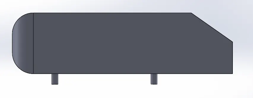
The Ahmed Geometry was prepared using Solidworks. The exact dimensions were used in order to get a good result.

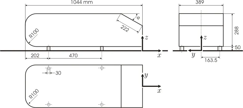
Ahmed Body can be downloaded from here: Ahmed body

Various Features were used to create the geometry like a sketch and extrude.

Isometric View

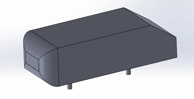
*The Slant angle was kept as `35^o` that is also called as Critical Angle

Front View and Side View

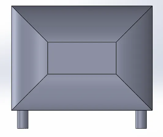
Case Study Set-Up

1.Geometry Creation

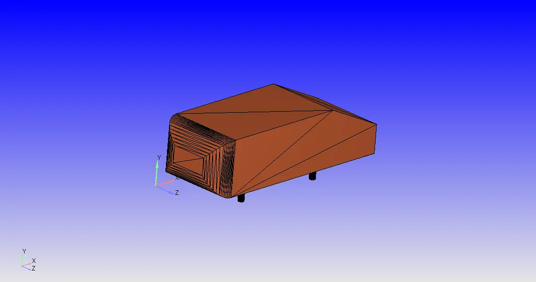
First of all, the Ahmed body geometry was imported using converge CFD software. The geometry was separately prepared using different CAD package ie Solidworks, then .stl file was imported to Converge Studio to set up the case study. The exact dimensions were used to create the geometry. After importing Ahmed body, a Virtual wind tunnel was setup using proper dimensions.

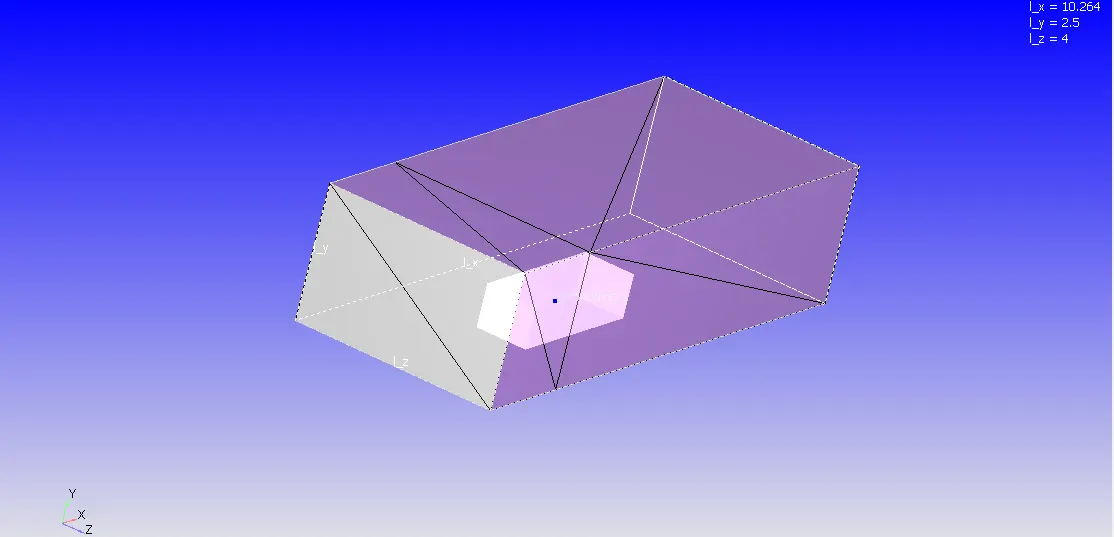
The Virtual Wind Tunnel Dimension is :

Dx(m)	Dy(m)	Dz(m)
10.264	2.5	4

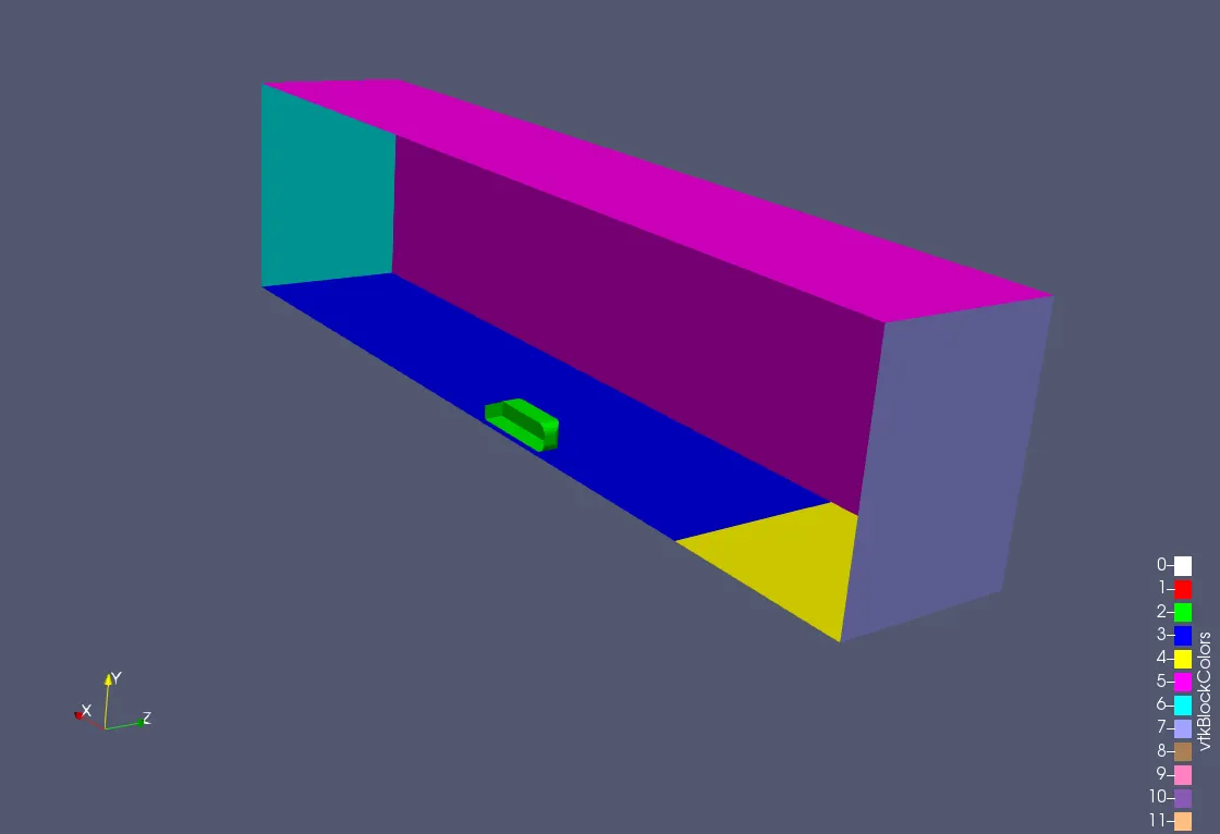
Inlet	Grey
Outlet	Green
Symmetry Wall	Pink
No-Slip wall	Blue
Slip Wall	Yellow
Ahmed Body	Green(Leaf color)

The Slant angle was kept as `35^o` That is also called as Critical Angle.

To create the geometry, the geometry was uploaded from the different CAD software package. All the normal vector were pointing out for this geometry, so we wanted it to point inside and normal to each surface. Normals point the direction of the fluid region generally. The command "Transform" was used to make the normal inside pointing the direction of the fluid region.

2.Boundary Creation

After creating the Ahmed body along with Wind Tunnel Geometry, The Boundry tag was created along with different boundary id and coloring. A total of 6 different boundaries tag was created for multiple different split triangles of the geometry with each face split into multiple triangles. To create the boundaries naming, the "Boundary" command in the "Geometry" dock was used, and then the faces were appointed to appropriate tags along with id.

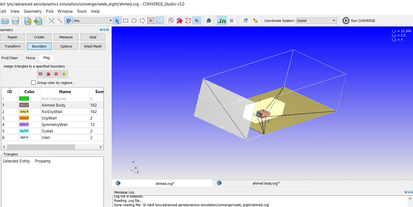
The six different boundaries were Inlet, Outlet, AhmedBody, NoslipWall, Slipwall, and SymWall.

3.Case-Study Setup

The various parameter was considered while setup this case study. The case study setup dock was used to set up the problem which appears on the right-hand side of the converge studio.

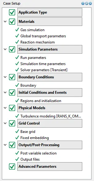
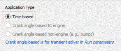
3.1 Application Type:

In order to run a steady-state simulation, firstly, under the Application type in the setup tree, a "Time-based" simulation must be selected.

3.2 Materials:

Under the material tab "Gas simulation" was selected and "Air" as a predefined mixture.

Gas: Air

Global Transport Parameters: Fixed value

by default, the following value is considered.

Prandtl Number : 0.9

Schmidt Number : 0.78

Species: Oxygen-O2 & Nitrogen-N2

3.3 Simulation Parameters

The Transient solver was selected for running this case study along with a "Density-based" solver.

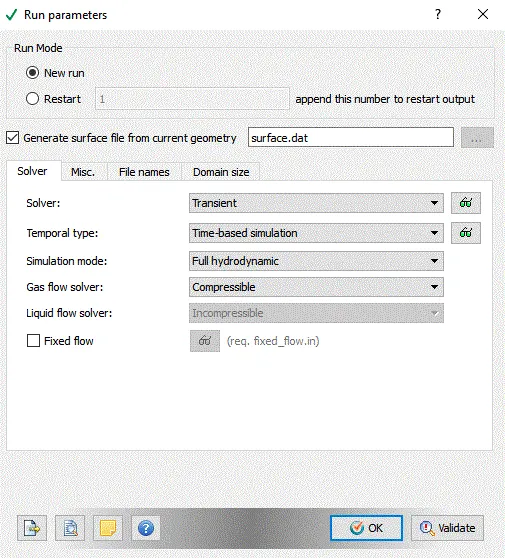
Calculation

Horizontal length=10.264m

Average Velocity=40m/s

Speed=Distance/time

therefore, Time=0.2566 sec

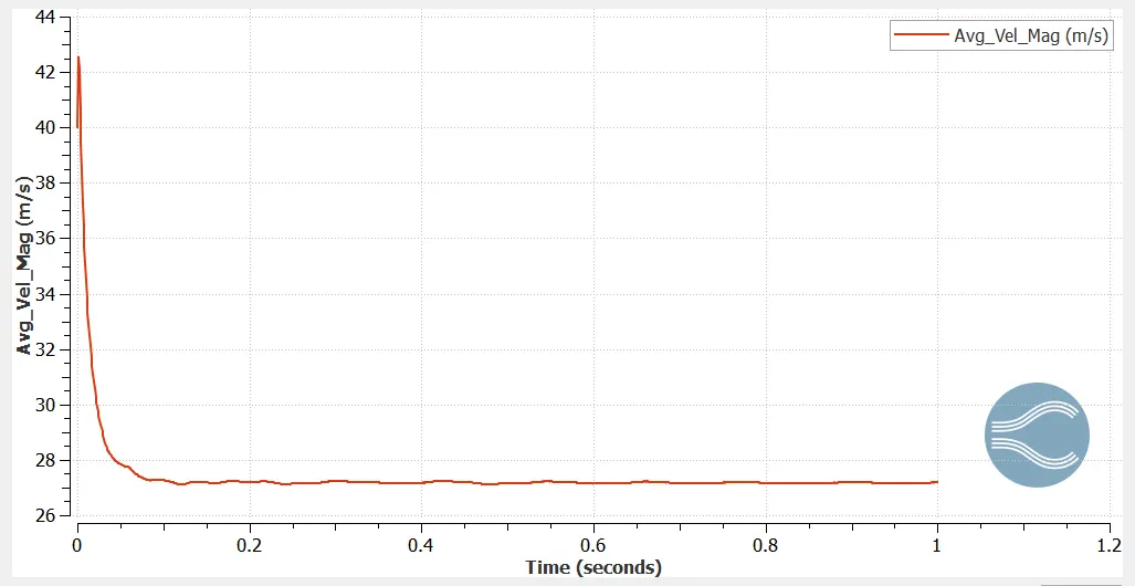
we are simulating roughly 4 times of flow through time that is 1s

The Following Simulation parameters were selected for running this simulation.

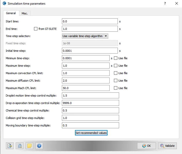
3.4: Boundary Conditions

In this tab, The volumetric region and physics for each boundary were defined.

Boundary_Name	Boundary_Type	Paramter_Defined	Boundary ID
1. AhmedBody	Wall	Law of Wall	1
2. NoSlipwall	Wall	law of Wall	2
3. Slipwall	Wall	Slip wall	3
4. Symmwall	SYMMETRY		4
5. Outlet	Outflow	101325.0 Pa at 300 k (Dirichlet Boundary Condition)	5
6. Inlet	Inflow	40m/s in X-axis (Dirichlet Boundary Condition) The pressure being at NE (Neuman Boundary condition)	6

3.5: Initial Conditions and Events

Volumetric Region was created in order to assign this to all the boundary tag.

Species:- O2 (0.23) & N2 (0.77)

Pressure :101325Pa

Temperature:300K

The velocity of 40m/s in X-axis

3.6: Physical Models

A turbulent model was selected out of so many models.

This turbulence model is the combination of RNGl-E and Standard K-Omega and hence it near the wall "K-Omegasst" works as a standard k-omega model and away from the wall, it works RNGk=e model. Hence it gives an accurate prediction near the wall and away from the wall, as we are intersecting in capturing boundary layer growth.

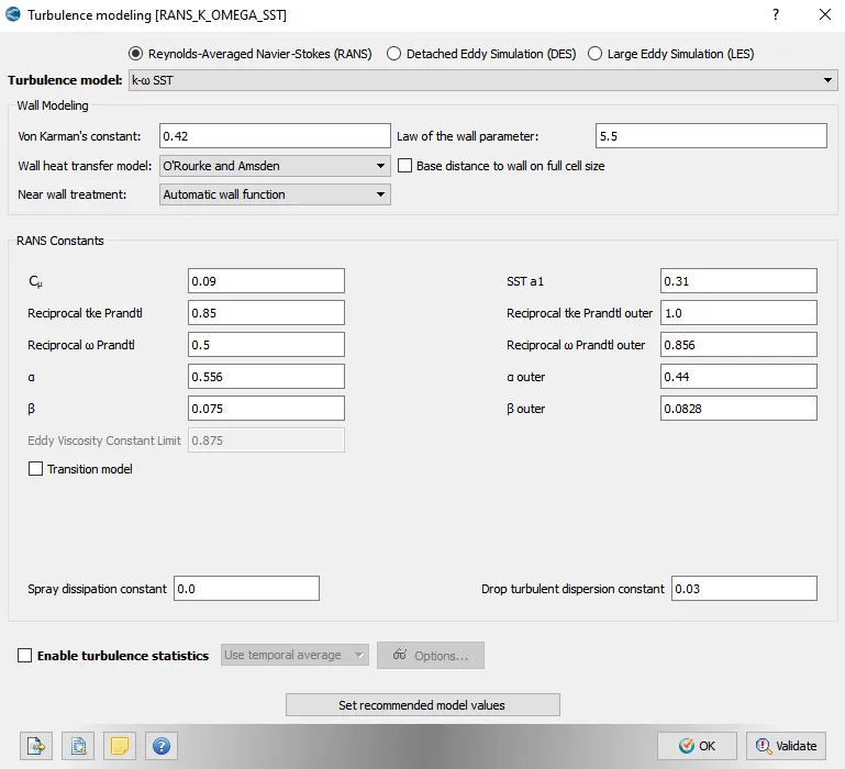
3.7: Grid Control

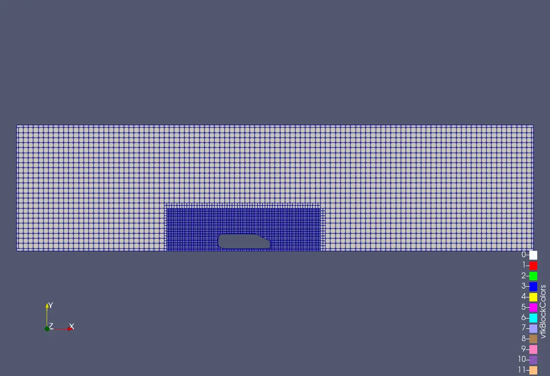
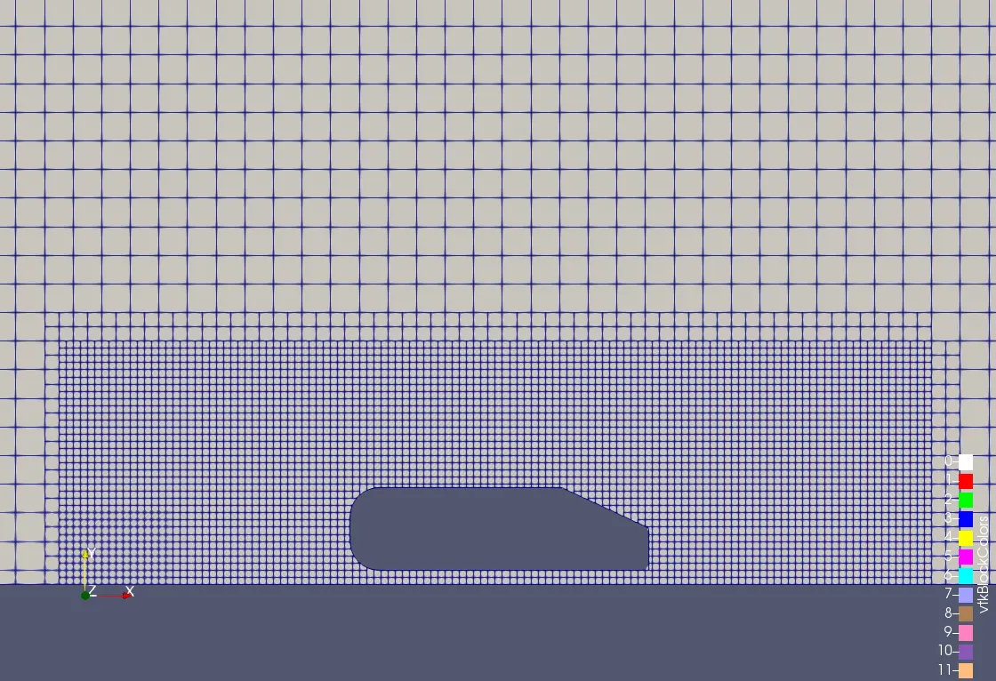
The case study was run using a Coarse mesh grid size due to less computational resources.

Base mesh sizes are,

S.No.	Dx(m)	Dy(m)	Dz(m)
1	0.09	0.09	0.09

Fixed embedding was done in order to capture more cells near to throttle in order to get more precise data.

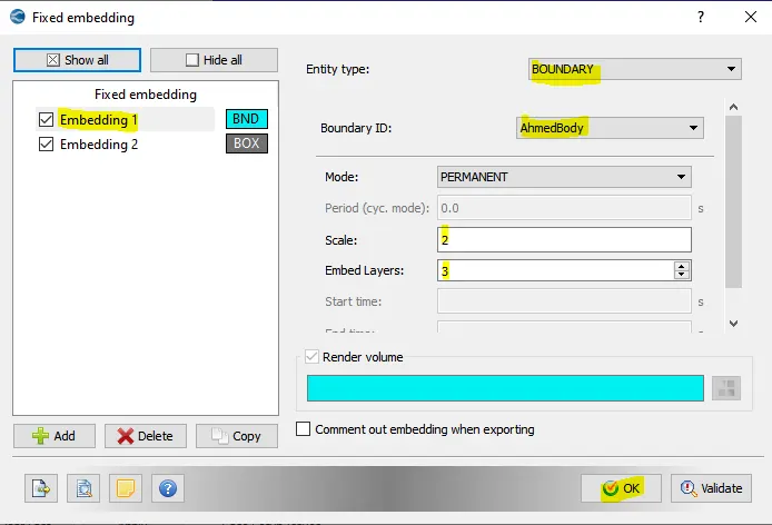
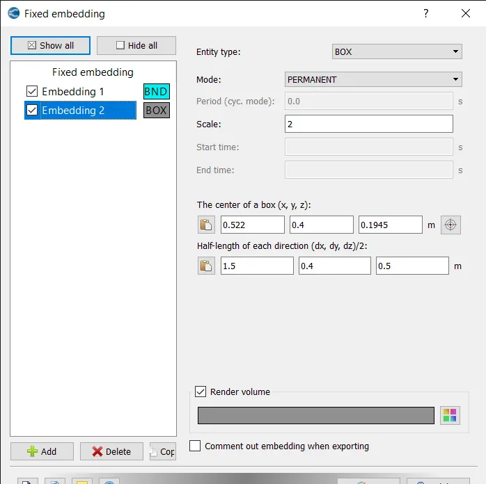
Wind tunnel that has box embedded inside with more fine computational cell in order to capture more data more precisely

3.7 Output/Post-Processing

In regions and initialization, the value of velocity should be the same as that of Inlet velocity.

Also, while setting up the case, make sure, wall output (BOUNDARIES ONLY) is enabled as this will dump wall averaged output data which is very much important for any external aerodynamic simulations.

Post-Variable Selection- Existing value

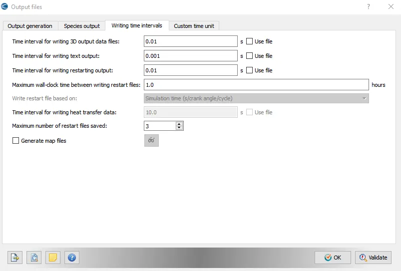
Output Files- Time interval for writing 3D output files-0.01 s

The time interval for writing restart files -0.01s

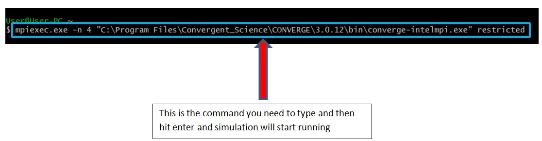
The case study was solved using CYGWIN and the post-processing was done in ParaView.

Simulation Results

Mesh Model

Converge Plots

Velocity Plots

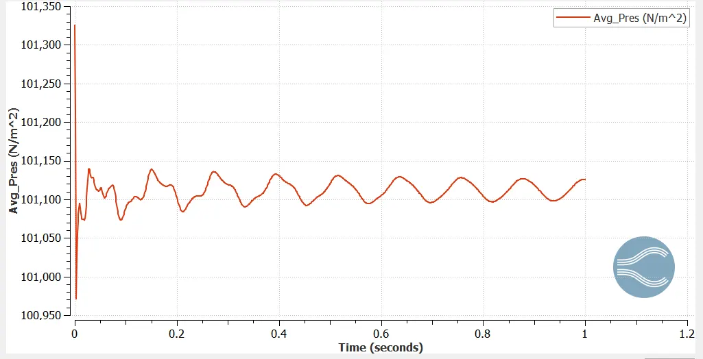
Pressure Plot

Contours

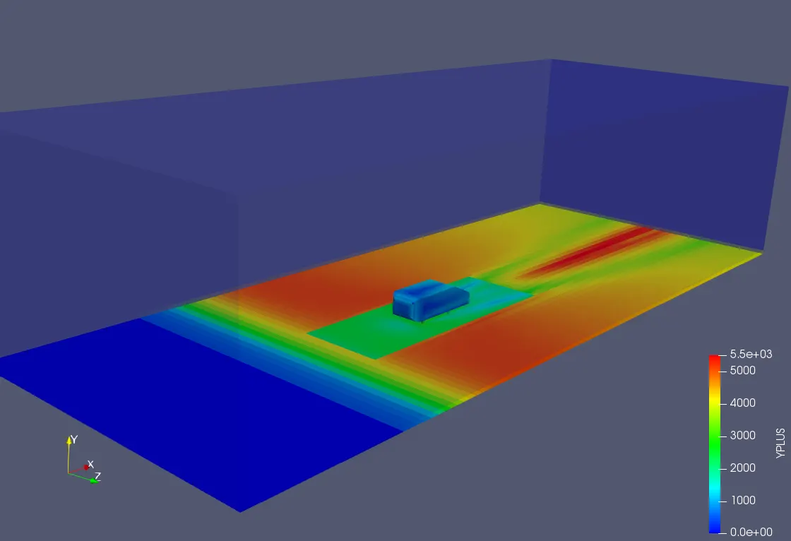
Y plus Contours

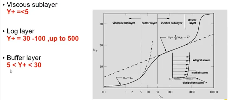
Turbulence is the state of chaotic and unstable fluid flow, just opposite of Laminar flow. Y plus(Y+) is the non-dimensional distance of the first cell from the wall.

Let's takes an example of a flat plate under zero pressure gradient and front left side the uniform velocity is coming to the plate. Firstly, it will be laminar flow, then after some disturbance, the region will be called as Transition Region, when the disturbance is growing too much the flow will change in Turbulent Flow. The boundary layer in the turbulent region will be called a turbulent boundary layer whereas in laminar it will be called the laminar boundary layer.

Reynold's Number Re">ReRe is the ratio of Inertial force to the Viscous Force.

Viscous Sub Layer: Viscous stress term dominates

Buffer Layer: Transitional region

Log law Region: Reynolds shear stress term dominates

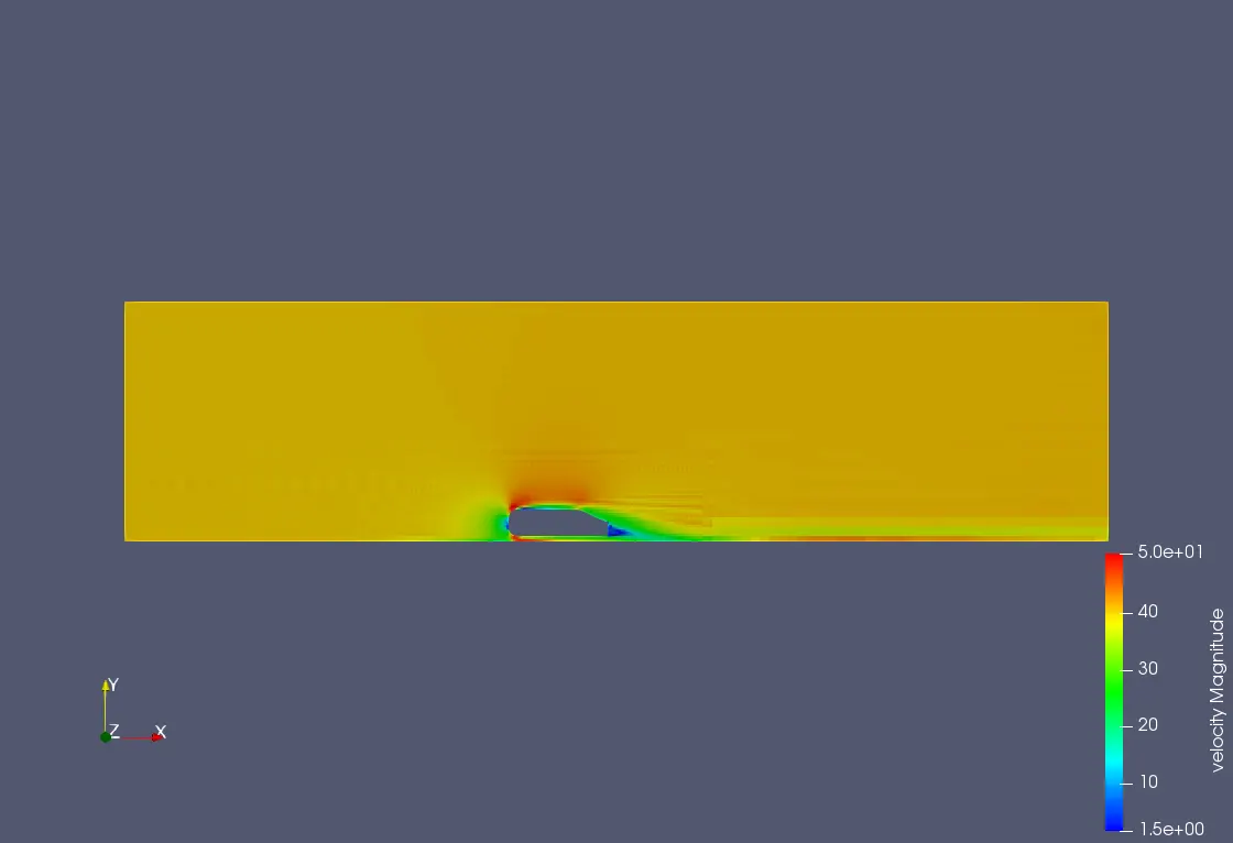
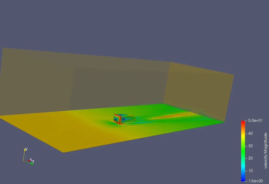
Velocity Contour

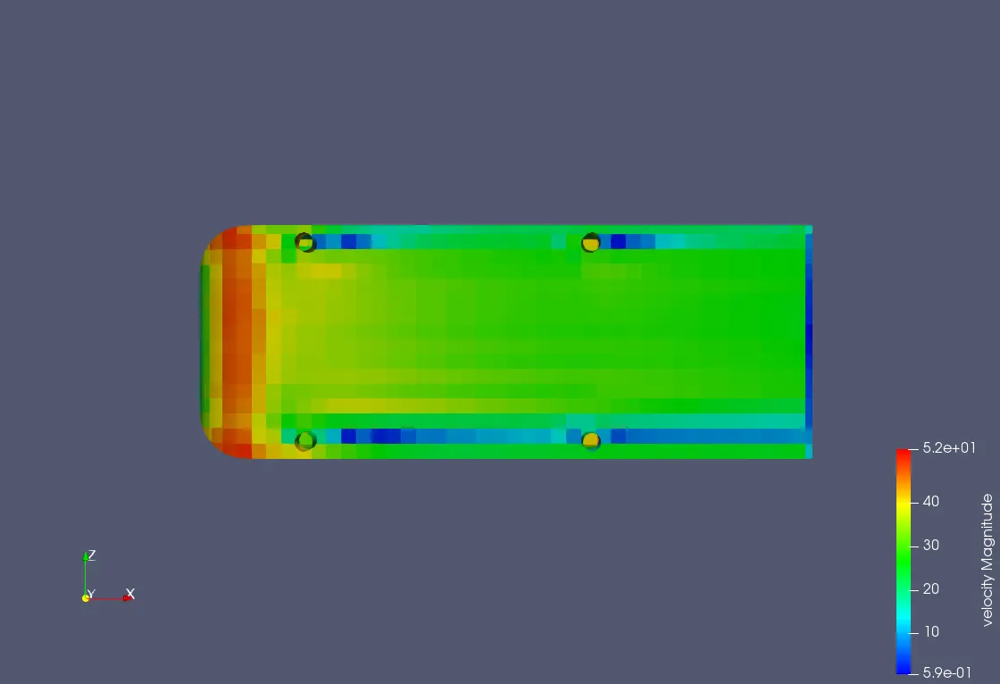
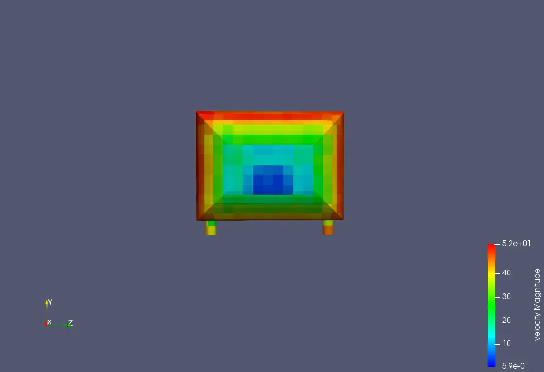
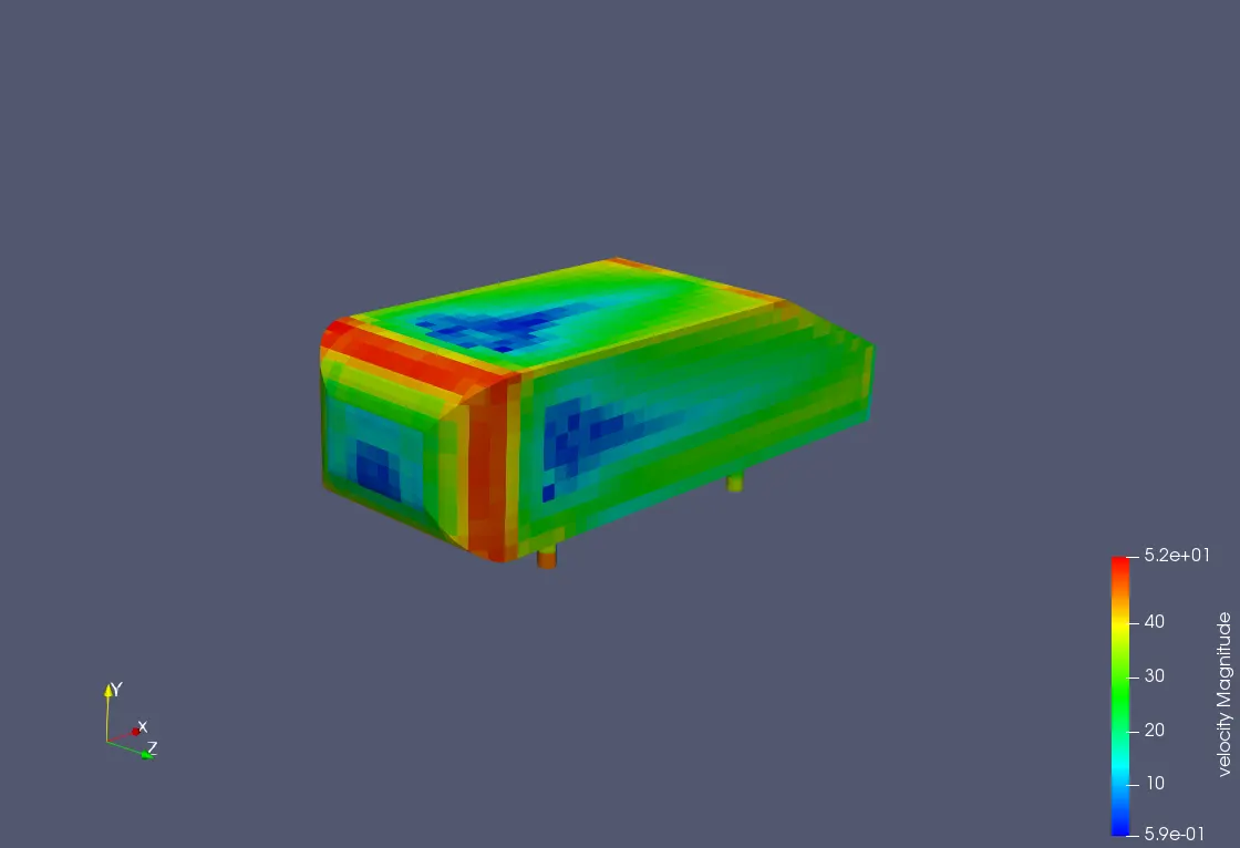
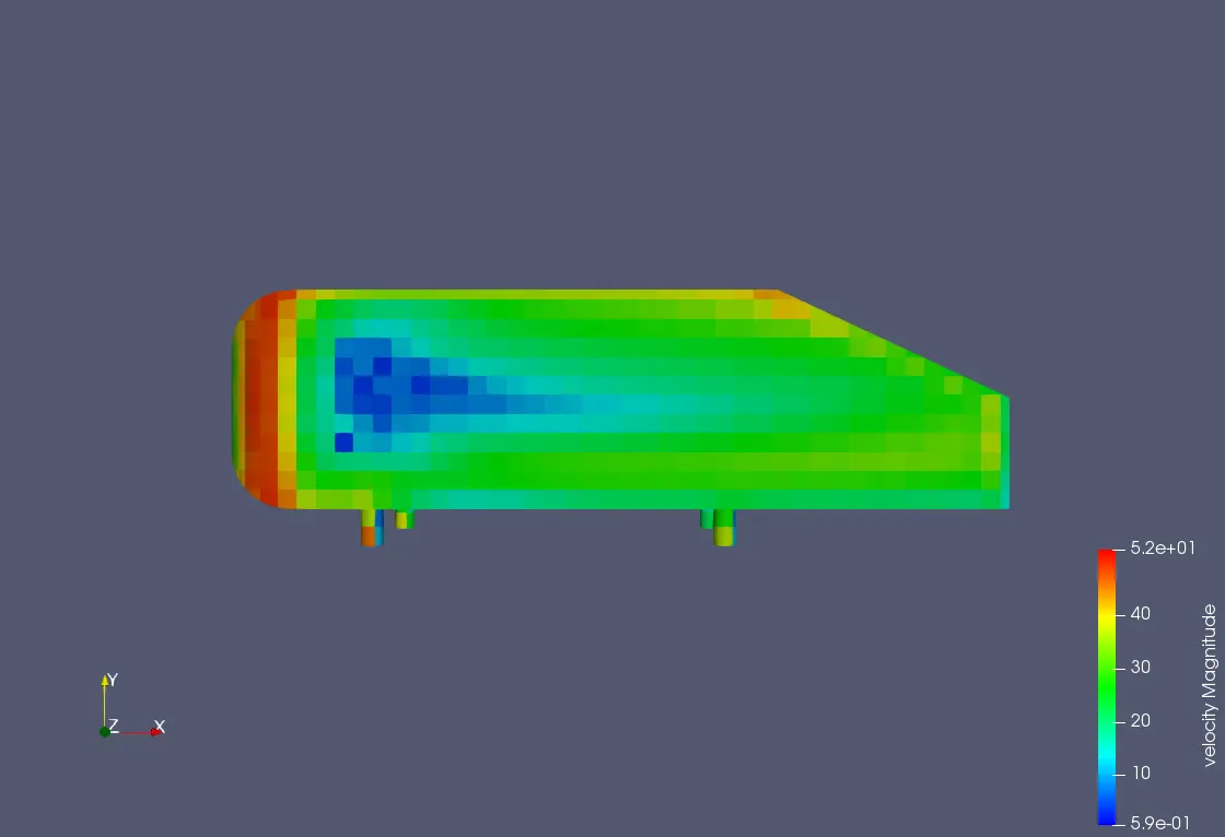
Observation

The velocity at the backside(indicated in blue color) is very low and there is a formation of the recirculation zone the top and side surface of Ahmed's body has a layer of very high velocity along with high pressure. then due to slant, the flow is getting separated along with the formation of recirculation.

The Velocity is very low in the windward side because the airstrikes the front area and losses its kinetic energy. The low-velocity region along the trailing edge is called the wake region, which is due to the slant angle of Ahmed's body i.e.35 deg. it is accorded to the geometry. this seems to move because the vortices formed in the region due to the recirculation of air. This contributes to the majority of the drag force on the body as it causes suction to take place in the location which ultimately adds up the drag on the body.

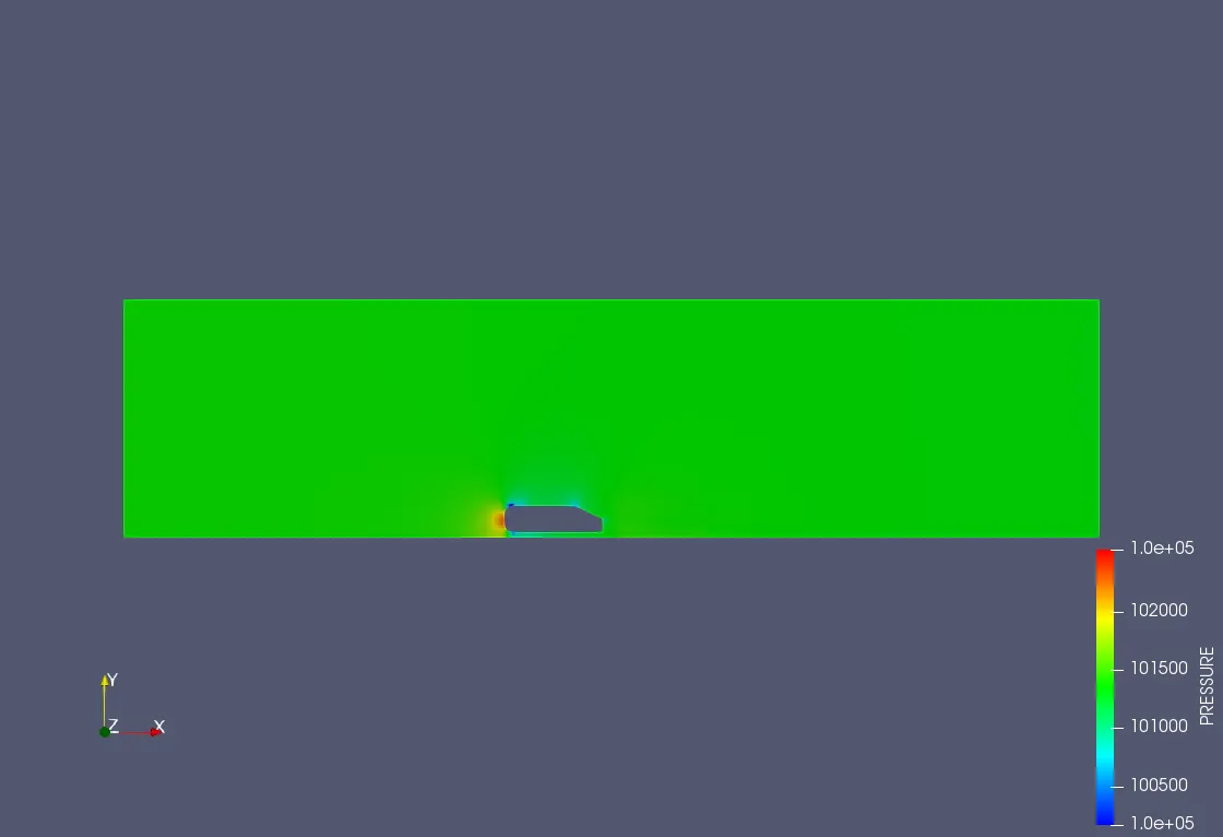
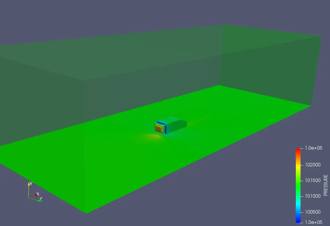
Pressure Contour

Flow Lines

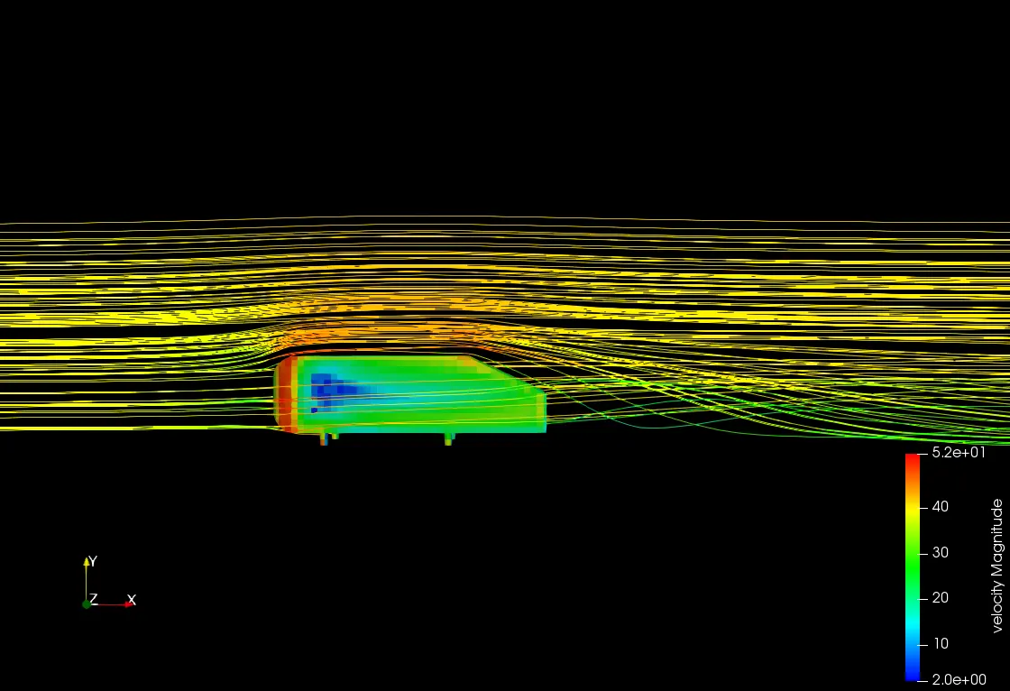
The flow is diverted to a greater extent by the front surface as it comes are rounded. The nature of flow in the lower side is due to wake formation, which is due to flow separation and recirculation.

Observation

The pressure is very high on the front face of Ahmed's body due to flatness its because the wing is hitting that surface and forming a high-pressure zone indicating in the red zone.

The pressure becomes a bit lower on the top and sidewalls of Ahmed's body and has a little bit of high pressure as compared to the backend of Ahmed's body that has very low pressure because the wing losses its kinetic energy. As the airstrikes, the front surface the kinetic energy becomes low which results in loss of pressure as well as velocity. The pressure is known as stagnation pressure. the flow separation takes place at the sharp ends which is responsible for wakes formation and also responsible for pressure drop

---------------------------------------------------------------------------------------

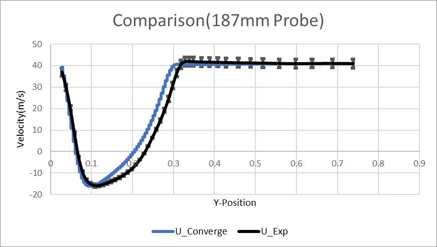
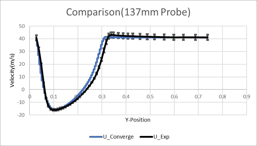
Velocity in X-axis along with different Z location

The Values of experimental data was provided and we need to compare those result with the simulation data obtained.

• 
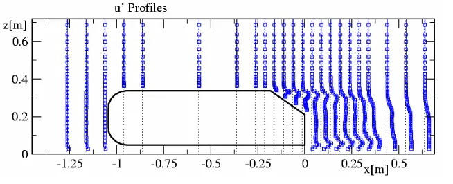
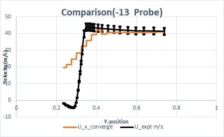
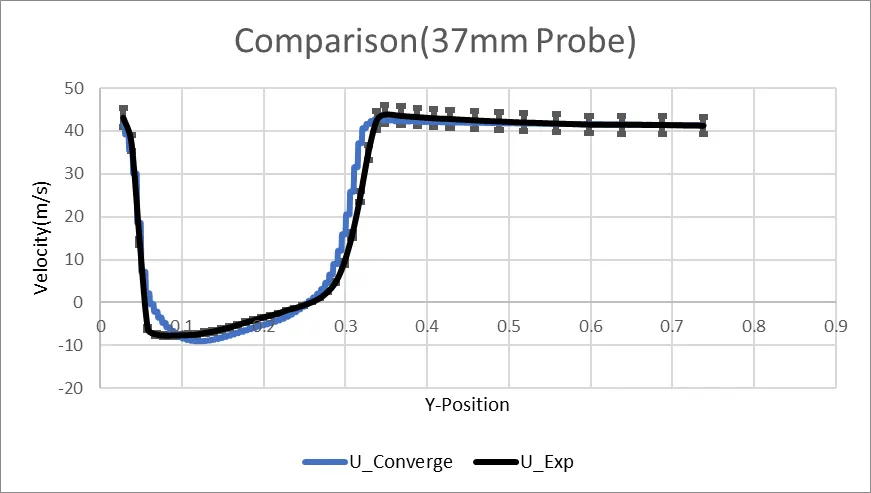
• As the probe is near the rear end, there is reduction in velocity for some length. The experimental data and the simulation data have a similar trend, though don't coincide which is accorded to the coarse meshing due to the system constraints.
• 
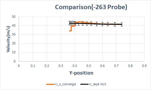
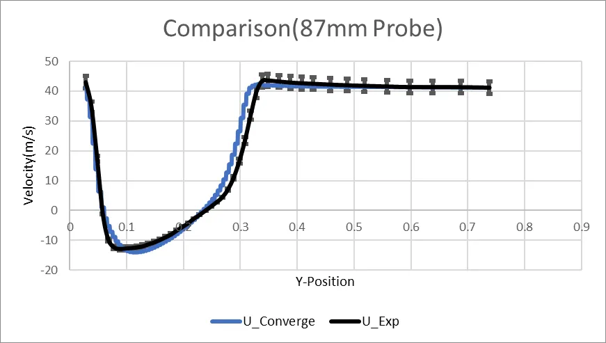
• As this one is quite away from the rear end, the velocity is a bit steady. The experimental data and simulation data coincide to a greater extent, as this area is not critical to changes.
• 
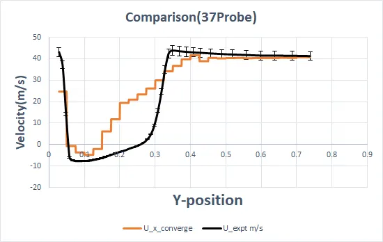
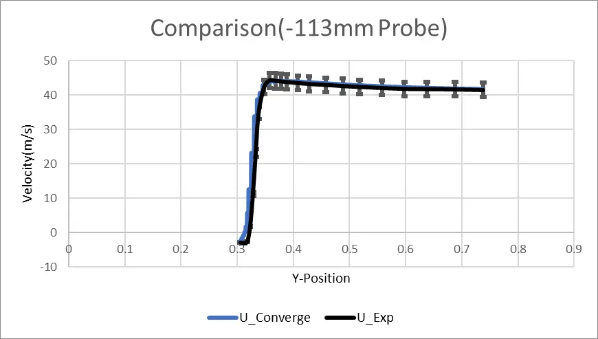
• This is placed in the wake region, so the velocity is negative at certain locations. Again, both the data possess a similar curve trend, which suggests that the simulation is valid.
• 
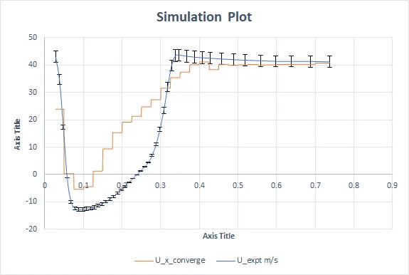
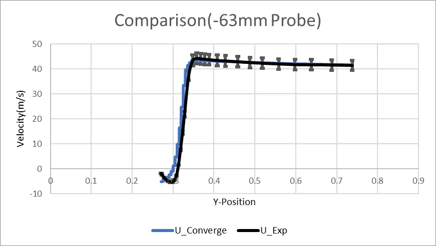
• Similar to the previous one, even this is placed in the wake region, as the velocity is negative. Again, both the data possess a similar curve trend, which suggests that the simulation is valid.
• 
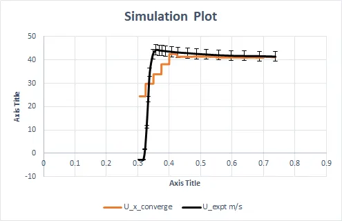
• This is closer to the rear end, where flow separation takes place, hence the above plot is got. Though the curves have a similar trend, the velocity near the walls don't coincide.
• 
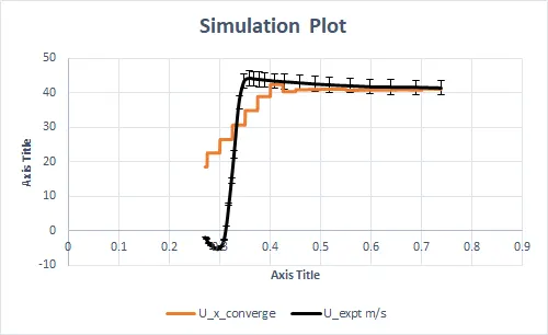
• Similar to the previous one, even this is plsce in the flow separation region. Though the curves have a similar trend, the velocity near the walls don't coincide.
• 
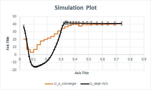
• It is placed in the wake region, which results in the above plot. The data possess a similar trend, hence the simulation is valid.
• 
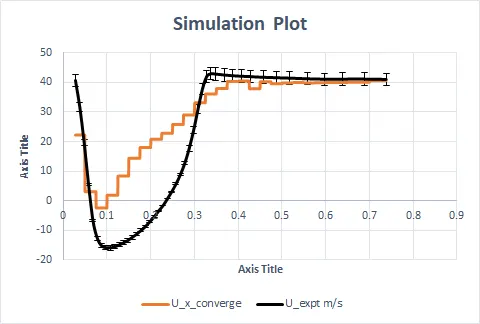
• This is again similar to the previous plot. The data possess a similar trend, hence the simulation is valid.
• Therefore, the overall simulation is found to be valid as the trends of the curves match eachother. The deviation in a certain curves are accorded to the coarse meshing.
• The below are the plots made from the simulation with high degree of refinement.

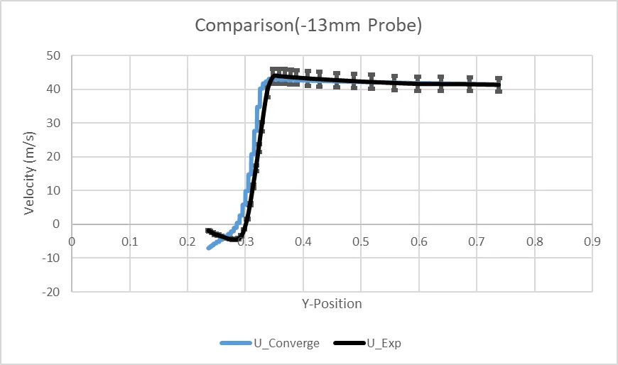
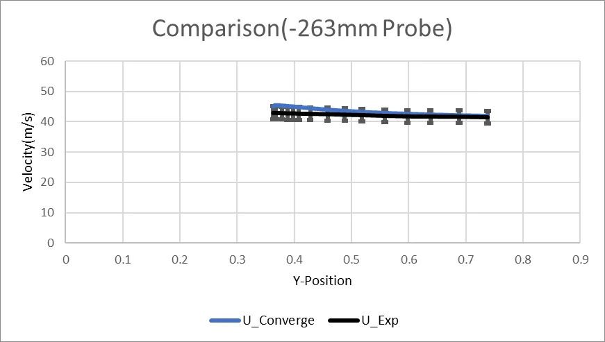
• • The above plots coincide well with the experimental data as the refinement is higher.
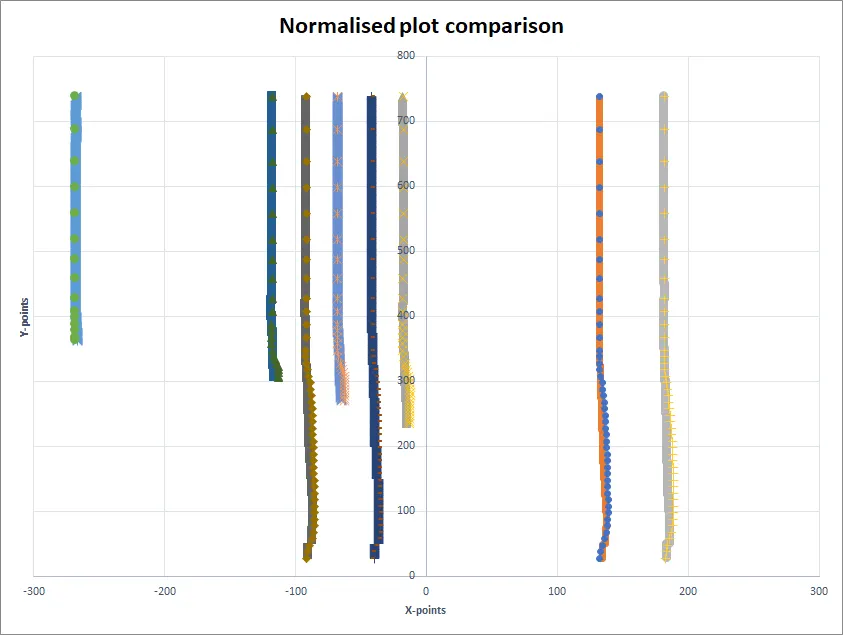
• Normalised Velocity Plot:
  • Normalisation is done to visualise the velocity profile and compare it a bit easily. In order to normalise, for each line probe (both experimental and simulation data), the velocity at each point in the line probe is divided by the maximum velocity along the line and multiplied by an amplification factor, here 5. Then this value is subtracted from the x-coordinate value of the line, so that it could be plotted for comparison. The below plot shows the normalised velocity plot, which suggests that the simulation and experimental data coincide to a greater extent. This shows that the simulation is valid. (Note: For verification, the results of simulation run in a high configuration system have been included in the last)
  • Link for the Excel file containing all the data including normalisation:Datasheet

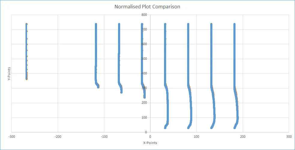
The Normalised plot obtained from the simulation with higher degree of refinement is shown below. The link for Excel file containing data and calculation pertaining to the refined simulation:Refined mesh Datasheet

Finding the Coefficient of Lift and Drag using ParaView:

ParaView is an important post-processing tool to visualize the results for Ahmed body. Various steps are followed in order to generate Lift and Drag force.

1. First the test.vtm files was imported in Paraview. The .Vtm was created using a converge studio using a post-processing dock.

2. The second step was to generate the Ahmed body so that the "Extract Block" Filter was used to generate the Ahmed body.

3. The third step was to generate the Surface of Ahmed body so a filter called "Extract surface" was used to extract surface for creating the surface normals.

4. Then the surface normals were created using the option in the filter.

5. Then the Lift and Drag force value was calculated using a Virtual calculator.

Lift Force(For single-cell) =PRESSURE*Normals_Z

Drag Force(For single-cell)=PRESSURE*Normals_X

6. Then the cell data was integrated using a filter called "Integrate Variable"

Converge Plot

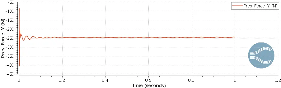
Lift Force

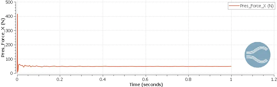
Drag Force

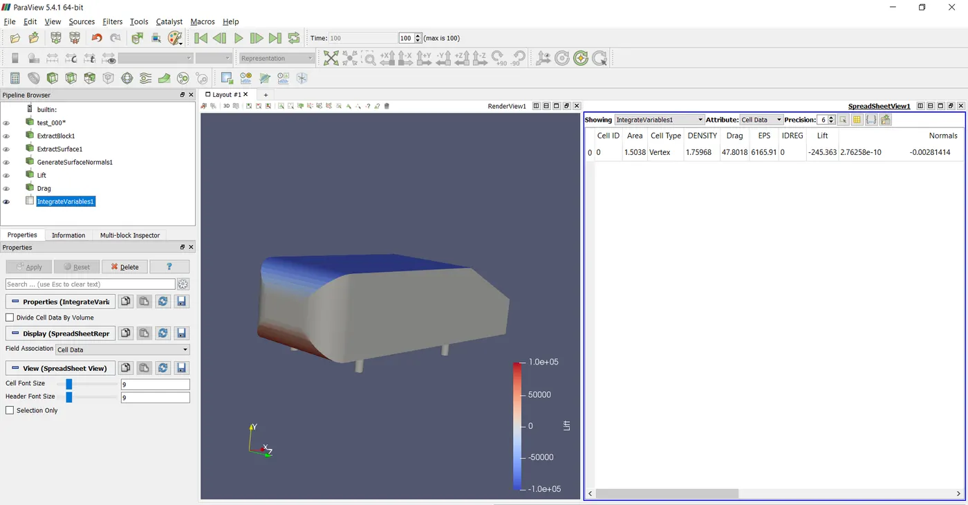
The Lift Force is found to be -245N

The Drag Force is found to be 47.80N

Fontal Area(A)=0.228x0.389

`rho=1.225(kg)/m^3`

Coefficient of Lift `C_L=(2*"Lift Force")/(rho*A*v^2)`

Coefficient of Lift `C_L=(2*(-245))/(1.225*(0.228*0.389)*40^2)`

Coefficient of Lift `C_L=-2.818`

Coefficient of Drag `C_D=(2*"Drag Force")/(rho*A*v^2)`

Coefficient of Drag `C_D=(2*(47.801))/(1.225*(0.228*0.389)*40^2)`

Coefficient of Drag `C_D=0.5499`

A tutorial video can be found from here to calculate lift and drag force: Link For lift and drag

Conclusion:

At last, it can be concluded that in order to get more accurate data the mesh should be finer but the computation time will increase because a lot of error can be seen in plots that were plotted for different z locations for different Velocity X. The normalized plot was created which was okay as the Experimental and simulation value were intersecting each other mostly.

The Value of Lift and Drag force from Converge and ParaView was found to be the same. These values were used to calculate the coefficient of lift and drag.

Coefficient of Lift `C_L=-2.818`

Coefficient of Drag `C_D=0.5499`

The surface below to Ahmed's body was kept as the Noslip wall is because we wanted to capture the vicious region. In the Velocity plot, a recirculation plot can be found just behind the Ahmed body where velocity drops and pressure also drops(the region where the slant surface finishes). The Maximum Pressure is found on the front curve surface regions.

This Case Study can be downloaded from here: Case File