Prandtl Meyer Shock problem
Prandtl Meyer Shock problem:
Aim:
The major objective of this project was to Simulate Prandtl Meyer Shock Problem Using Converge CFD & to study the Effect of the SGS parameter on shock location along with other useful data.
1. Simulate the SuperSonic and SubSonic flow through a duct which has a sharp corner.
2. Study the effect of Shock formation when the Parameter such as grid and SGS are changed.
3. Study the Effect of the SGS parameter on shock location
Introduction:
The report contains a detailed description of the Prandtl Meyer Shock Problem using converge CFD software, solving it using CYGWIN and post-processing the result using ParaView. Various steps are discussed in this report while making a case set up for this case study. This report contains a detailed description of the case study with grid sizing, line plots, the effect of SGS parameter, and contours.
Literature Review:
1)
- Boundary Conditions:
- Boundary conditions are most important for solving equations involved in CFD, FEA, etc.
- These specify the value of the objective function at their boundaries.
- There are basically three types of boundary conditions, namely:
- Dirichlet's Boundary Conditions,
- Neumann's Boundary Conditions,
- Robin or Mixed Boundary Conditions.
- Dirichlet's Boundary Conditons:
- The prescribed surface value of the objective function is given as the boundary condition.
- At the boundary,`phi="Constant"`, where `phi`is the objective function, `phi(t) or phi(x,y,z) or phi(t,x,y,z)`
- Examples: `phi(0)=0m, v(l)=0"m/"s, f(0)="50N/"m^2`
- Basically, this is used when the boundary conditions are specified directly.
- Neumann's Boundary Conditions:
- The prescribed flux value of the objective function is given as the boundary condition.
- At the boundary, `(dphi)/(dn) = "Constant", "where n-is the normal to the considered parameter,"(dphi)/(dn) =f(t)" or" (dphi)/(dn) =f(x,y,z)" or"(dphi)/(dn) =f(t,x,y,z)`
- Examples: `(dphi)/(dn)=0",for adiabatic boundary for heat transfer"`
- It is used for heat flux problems to specify the heat gradient variation along a direction, adiabatic boundary conditions, etc.
- Generally, this is used in circumstances where the boundary conditions are calculated by the solver and not specified directly.
- Robin or Mixed Boundary Conditions:
- As the name suggests, this boundary condition is a combination of Dirichlet's and Neumann's boundary conditions.
- The boundary condition includes both the surface and flux values in the form of an equation.
- At the boundary, `alphaphi + beta(dphi)/(dn) = gamma`
- So, from the above, it is clear that the Neumann's boundary condition is used for the problems when the actual value at the boundary can't be calculated and is calculated by the solver itself.
- Now, for supersonic flows the values of various parameters in the outlet boundary can't be calculated directly, so, the Neumann's boundary condition is used.
- In Prandtl Meyer Shock or Prandtl Meyer Expansion Fan, the flow is supersonic, hence Neumann's boundary condition is used.
Note: Prantl Meyer Expansion Fan is generated when the air with supersonic(or sonic) velocity is flowing over a sharp convex edge. The above figure shows the generation of expansion fan when a plate at an angle `theta` to the horizontal is incident with air of Mach number greater than 1, i.e. supersonic.
2)
- Shock Waves:
- Shock waves are formed when the source of sound or disturbance is moving with the speed of sound or more than that of sound in that medium.
- These are formed due to the constructive interference of the sound waves as the source moves.
Note: The above picture shows clearly how and when the shock waves are formed. In cases (a) and (b) there is no constructive interference of the sound waves, hence no shock. In cases (c) and (d), the disturbance wavefronts(sound waves) coalesce, which leads to the formation of shock waves.
- There are two types of shock:
- Oblique Shock
- Normal Shock
- There is another classification based on whether the shock is attached to the body or not:
- Attached Shock
- Detached Shock(or Bow Shock)
- Oblique Shock:
- It is the shock which is at an angle to the surface of the object.
- It is formed in cases such as, the flow over pointed objects or sharp concave corners(as shown in fig. (b) below).
- Normal Shock:
- It is the shock which is perpendicular to the surface of the object.
- The flow over an air-foil, flow thro' a CD nozzle(as shown in fig. (a) below) are typical examples of normal shock.
- Attached Shock:
- As the name suggests, attached shocks are those which are attached to the surface of the object.
- This classification is affected by the semi-vertex angle of the wedge or the object. If it is less than a paricular critical value, it becomes an attached shock (as shown in fig. (c) above).
- Detached Shock:
- Similarly, detached shocks are those which are not attached to the surface of the object.
- If the semi-vertex angle is more than the critical value, it becomes a detached shock or bow shock(as shown in fig. (d) above).
Note: Shock waves cause a major change in pressure, velocity, entropy of the fluid flowing past. As these changes are dynamic and drastic, the study of shocks has greater importance when it comes to Computational Fluid Dynamics.
3)
- Comparative study of Prandtl Meyer Shock Problem for different SGS Criterion:
In order to setup the Prandtl Meyer Shock Problem, the following procedure is followed:
- The geometry for setting up the simulation is downloaded and diagnosed for surface errors, etc.
- The boundaries are flaged accordingly like the inlet, outlet, etc.
- The Case setup for the simulation is done to specify the materials, simulation parameters,etc.
- Here the solver is a density based solver as the flow is compressible and a steady state simulation is set-up.
- The boundary conditions and initial conditions are specified such as, Dirichlet's BC for inlet with inlet velocity of 640m/s, Neumann's BC for outlet as specified in the above discussion on boundary conditions. Top and bottom walls are considered as slip walls.
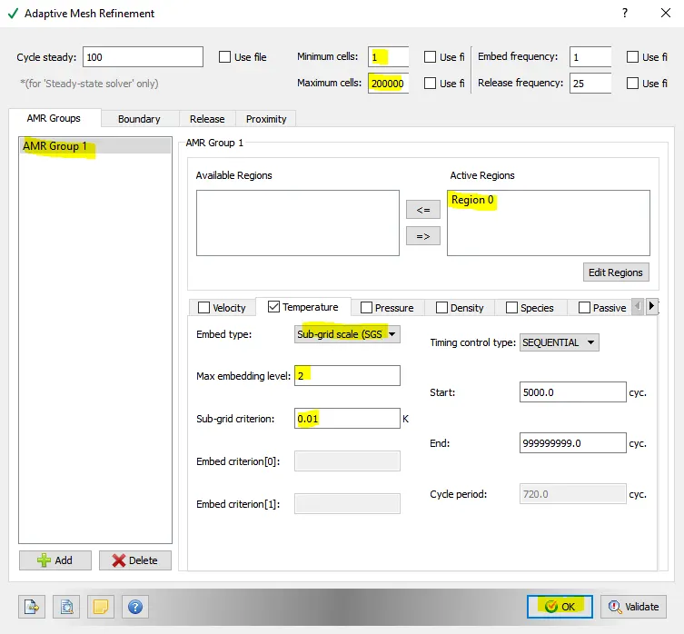
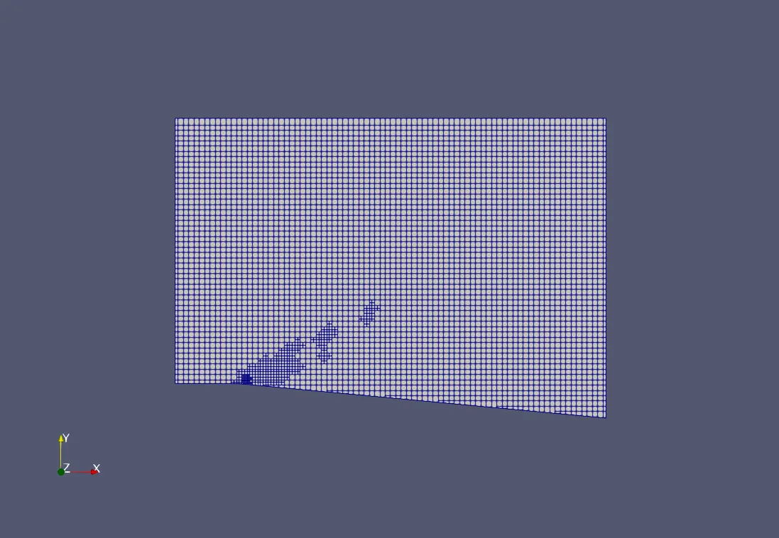
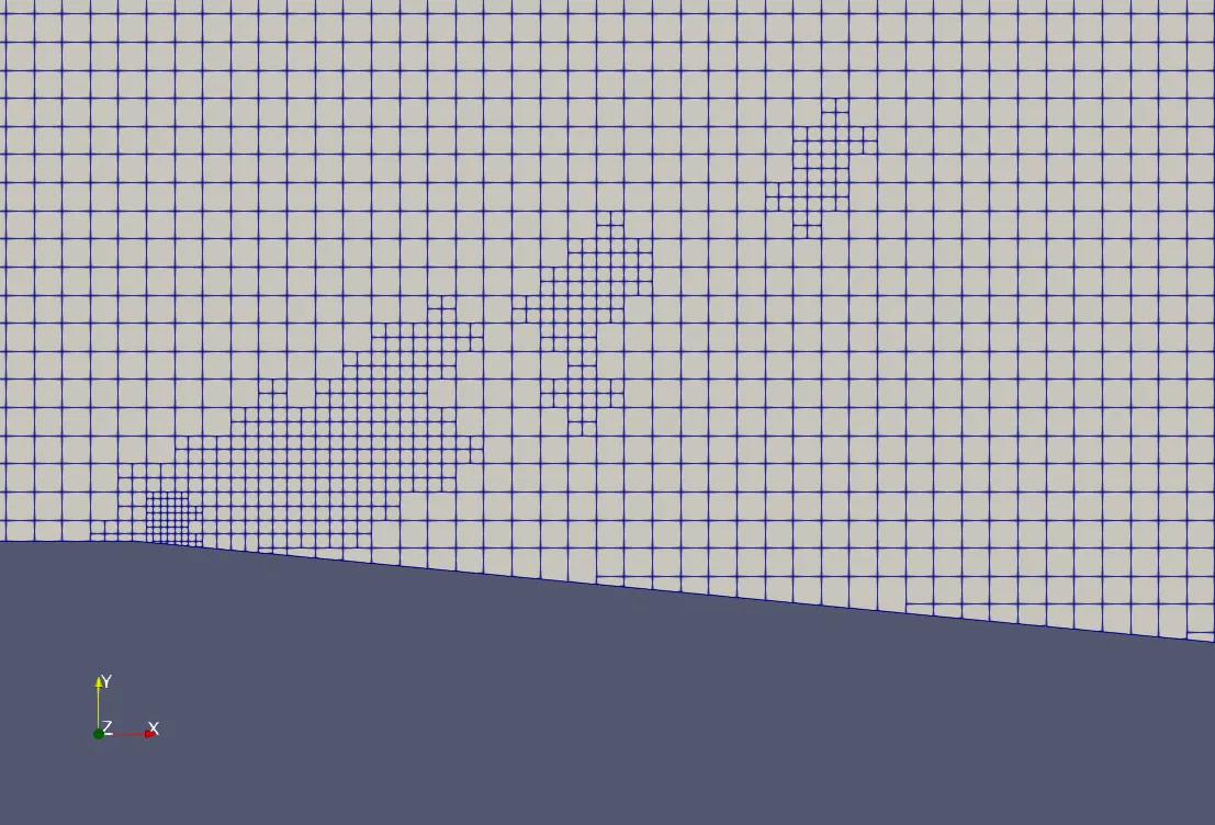
- The AMR(Adaptive Mesh Refinement) feature of Converge is used for meshing. This feature provides the advantage of automatic mesh refinement in certain places on satisfying a condition called the SGS(Sub-Grid Scale) criterion. This condition is specified based on the change in the gradient value of the parameter selected. It works in such a way that if the change in gradient is higher than the specified value, the mesh is refined further in those particular cells.
- Then the default parameters are set such as the output and post-processing, etc.
- Once the case setup is done the input files are exported.
- Then the Converge executable file is run and the output files are generated.
- The generated output files are post-processed and the inferences derived.
- The above steps are repeated for various SGS values(0.01,0.05,0.1).
Simulation setup:
1.Geometry Creation:
First of all, the Duct geometry along with sharp turn was imported in converge CFD software. The geometry was separately prepared using different CAD package ie. Solidworks, then .stl file was imported to Converge Studio to set up the case study.
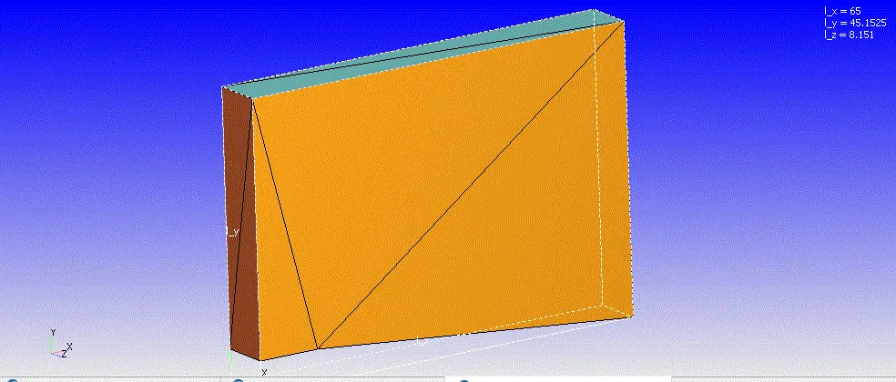
Image 1: Duct geometry along with Sharp corner.
*Each face of the step was split into multiple triangles.
The Geometry can be downloaded from this link: Geometry
To create the geometry, the geometry was uploaded from the different CAD software package. Then the geometry clean up was done along with inlet and outlet patch creation. All the normal vector were pointing out for this geometry, so we wanted it to point inside and normal to each surface. Normals point the direction of the fluid region generally. The command "Transform" was used to make the normal inside pointing the direction of the fluid region.
The Geometry was a check for if the geometry has any open surface.
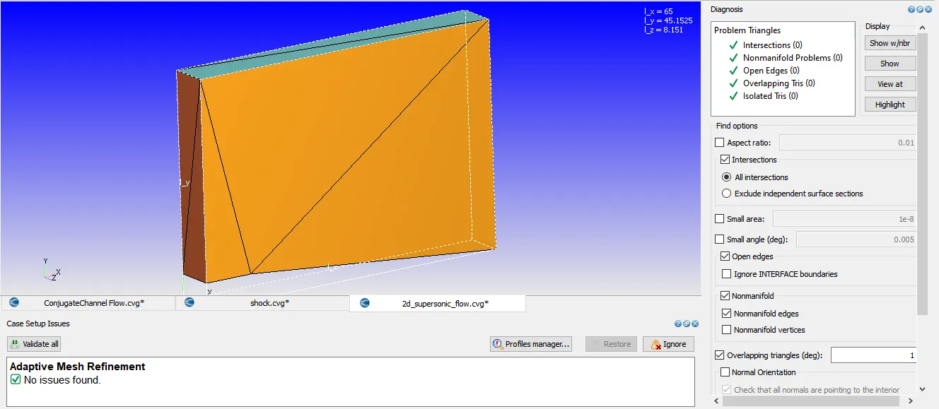
Then the normal edge checked and from the diagnostic dock, everything was checked.
2.Boundary Creation:
After creating the Duct Geometry, The Boundry tag was created along with different boundary id and coloring. A total of 5 different boundaries tag was created for so many different split triangles of the duct with each face split into multiple triangles. To create the boundaries naming, the "Boundary" command in the "Geometry" dock was used, and then the faces were appointed to appropriate tags along with id.
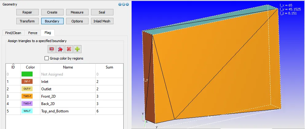
Image 2: Boundary creation representing the different id and color.
The five different boundaries were Inlet, Outlet, Top_and_Bottom, Front_2D, and Back_2D.
3.Case-Study Setup:
The various parameter was considered while setup this case study. The case study setup dock was used to set up the problem which appears on the right-hand side of the converge studio.
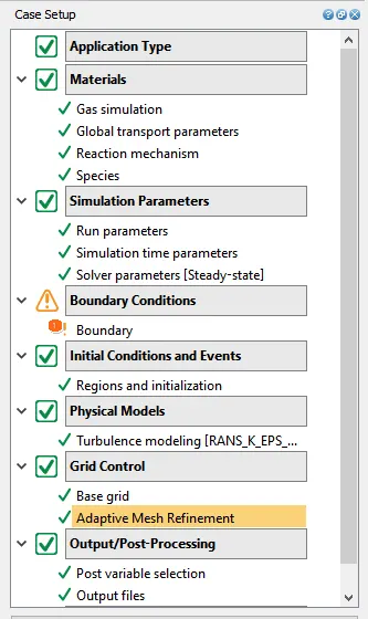
Image 3: Case Setup Dock.
3.1 Application Type:
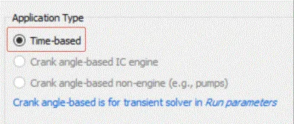
In order to run a steady-state simulation, firstly, under the Application type in the setup tree, a "Time-based" simulation must be selected.
3.2 Materials:
Under the material tab "Gas simulation" was selected and "Air" as a predefined mixture.
Gas: Air
Global Transport Parameters: Fixed value
by default, the following value is considered.
Prandtl Number : 0.9
Schmidt Number : 0.78
Species: Oxygen-O2 & Nitrogen-N2
Reaction Mechanism (mech.dat) was selected for this problem.
3.3 Simulation Parameters:
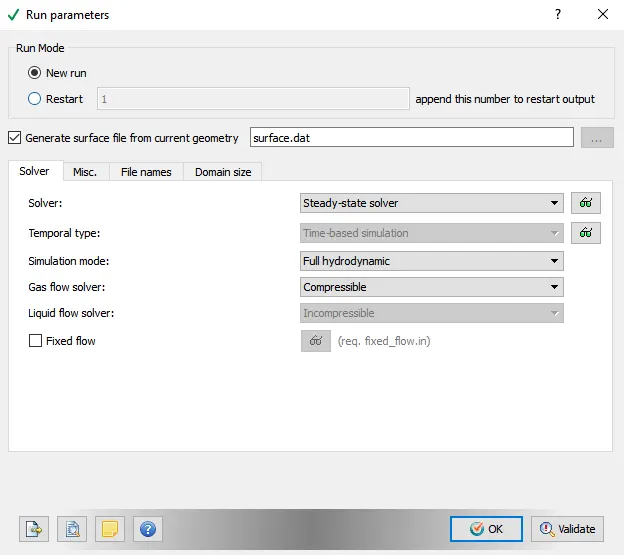
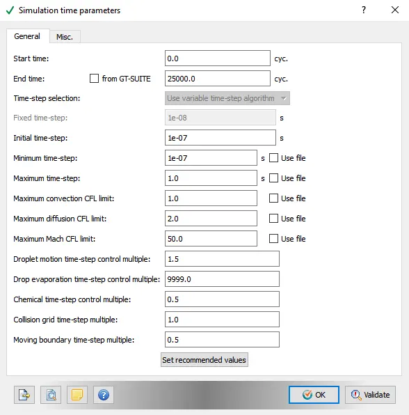
The Steady-State solver was selected for running this case study along with a "Density-based" solver.
3.4: Boundary Conditions:
In this tab, The volumetric region and physics for each boundary were defined.
| Boundary_Name | Boundary_Type | Paramter_Defined | Boundary ID |
| 1.Inlet | Inflow | 680m/s at 286.1k | 1 |
| 2.Outlet | OutFlow |
Dirichlet Boundary Condition Temperature Back Flow is 300K |
2 |
| 3.Front_2D | Two_D | 3 | |
| 4.Back_2D | Two_d | 4 | |
| 5.Top_and_Bottom | Wall | Slip | 5 |
3.5: Initial Conditions and Events:
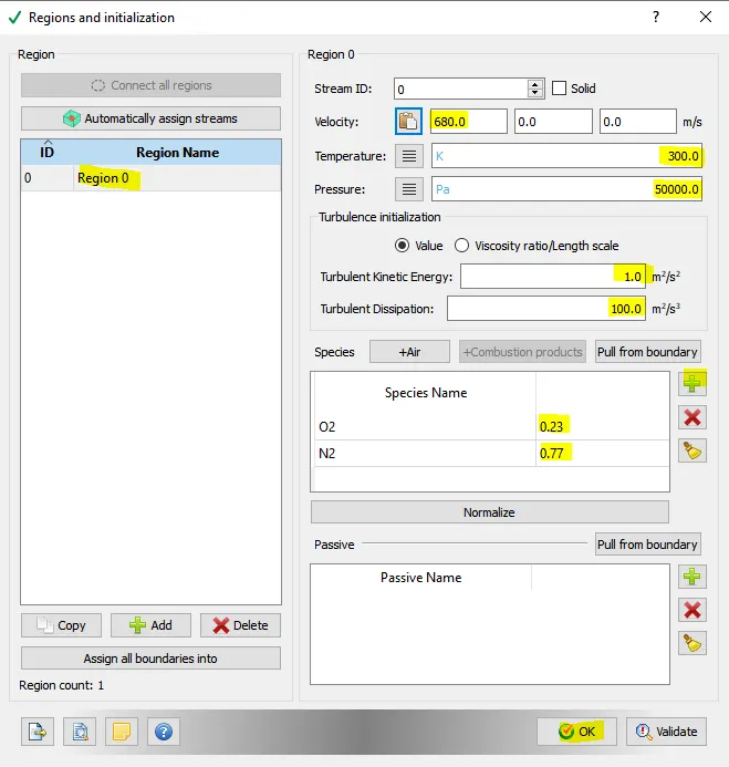
Volumetric Region was created in order to assign this to all the boundary tag.
Species:- O2 (0.23) & N2 (0.77)
Pressure :50,000Pa
Temperature:300K
Velocity:(680, 0, 0)m/s
3.6: Physical Models:
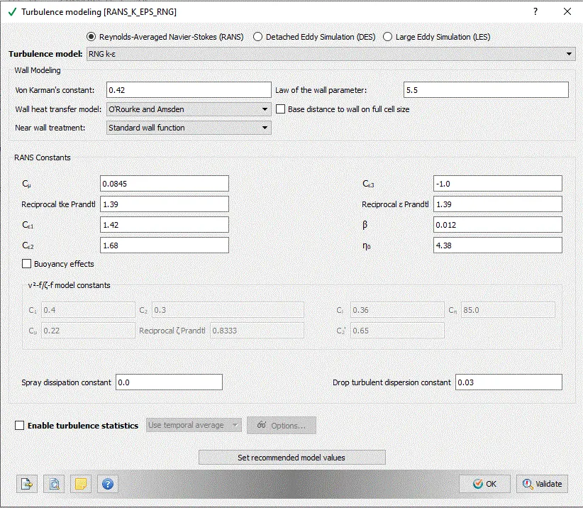
A turbulent model was selected out of so many models.
3.7: Grid Control:
The case study was run using a 4 fine SGS parameter size and at supersonic & subsonic speed. So different case study was set up in order to study the effect of value when the mesh is more refined.
The Adaptive mesh refinement was selected
Base mesh sizes are,
| S.No. | Dx(m) | Dy(m) | Dz(m) | Speed(m/s) | SGS |
| 1 | 0.8 | 0.8 | 0.8 | 680 | 0.05 |
| 2 | 0.8 | 0.8 | 0.8 | 680 | 0.01 |
| 3 | 0.8 | 0.8 | 0.8 | 680 | 0.1 |
| 4 | 0.8 | 0.8 | 0.8 | 100 | 0.05 |
3.7 Output/Post-Processing:
Post-Variable Selection- Existing value
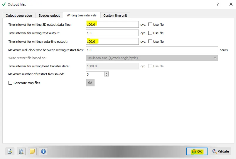
Output Files- Time interval for writing 3D output files-100 s
The time interval for writing restart files -100s
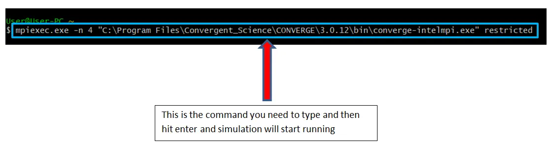
The case study was solved using CYGWIN and the post-processing was done in ParaView.
SuperSonic Flow:
Case Study 1: Grid Size 0.8m SGS 0.05 Velocity 680m/s
Generated Mesh:
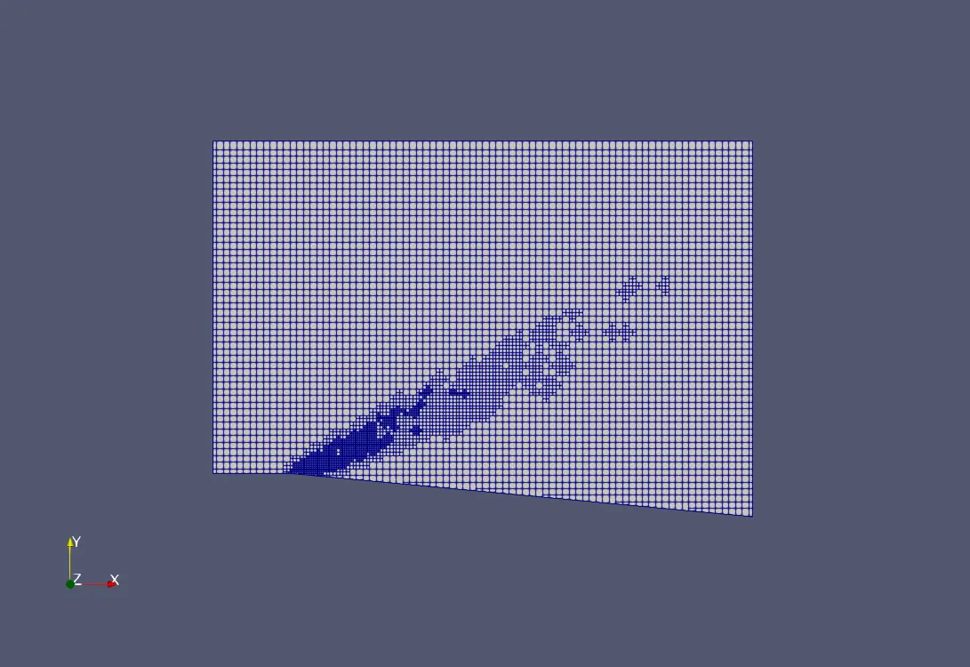
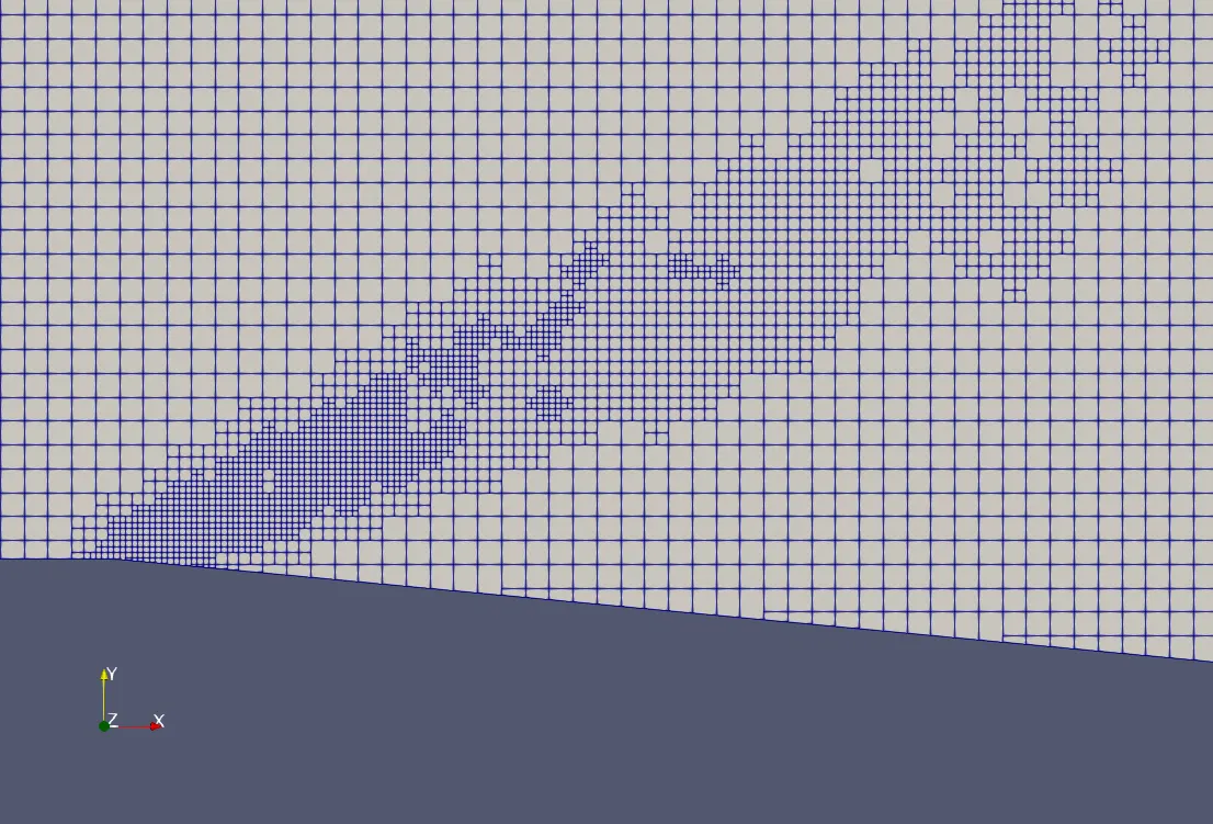
Result: (Line Plots & Contours):
1)Velocity contour and Plot:
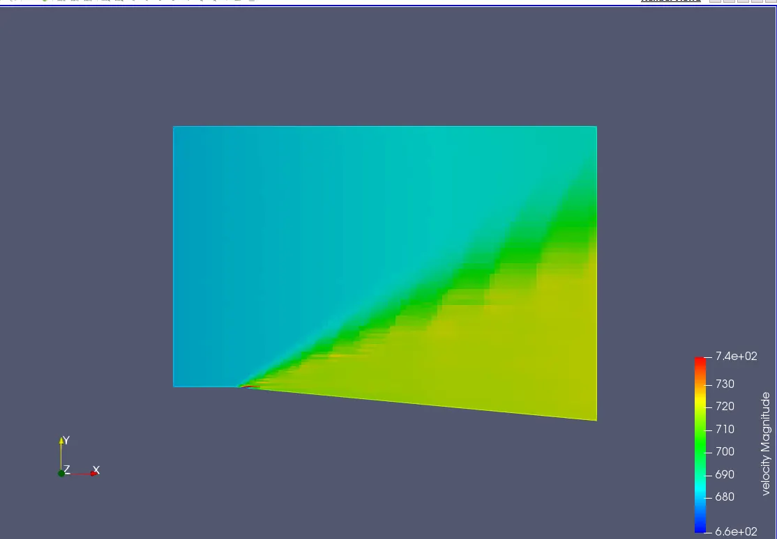
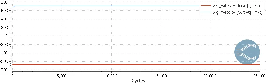
2)Pressure Contour and plot:
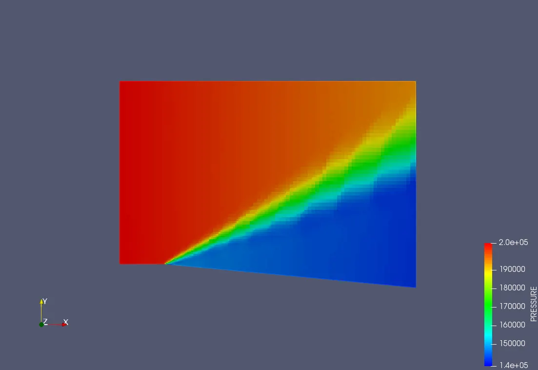
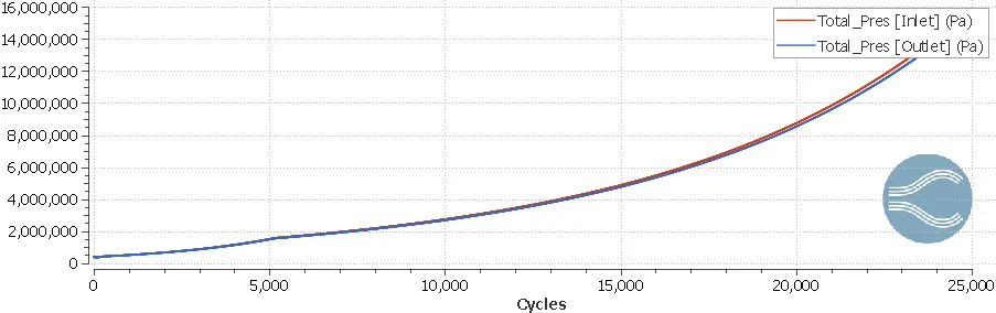
3)Temperature Contour and plot:
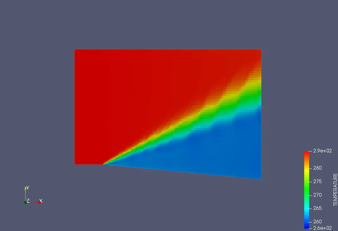
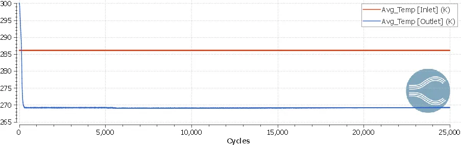
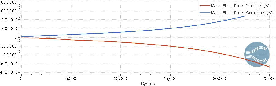
4)Average Mass Flow:
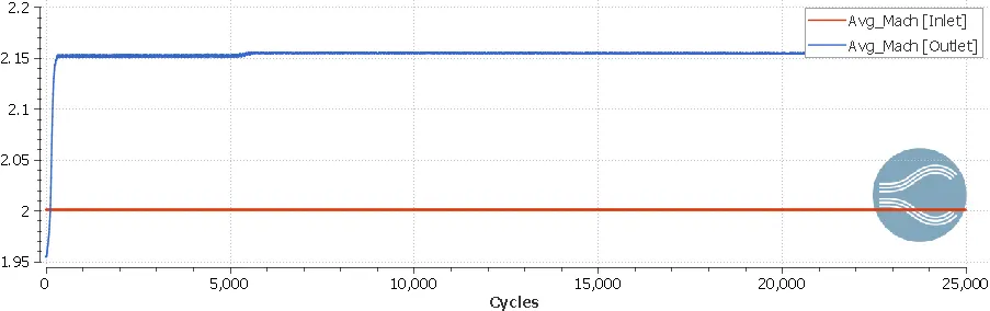
5)Average Mach Number:
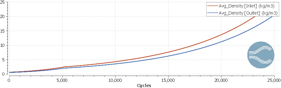
6)Average Density:
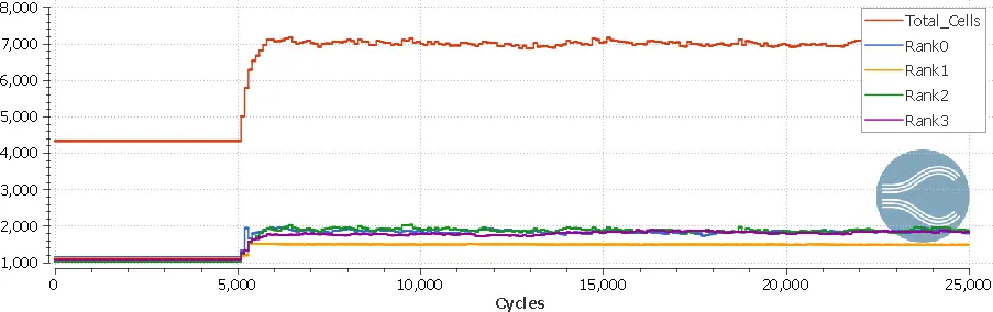
7)Total Cells:
The Youtube link for the animation of velocity,temperature and pressure contours are given below,
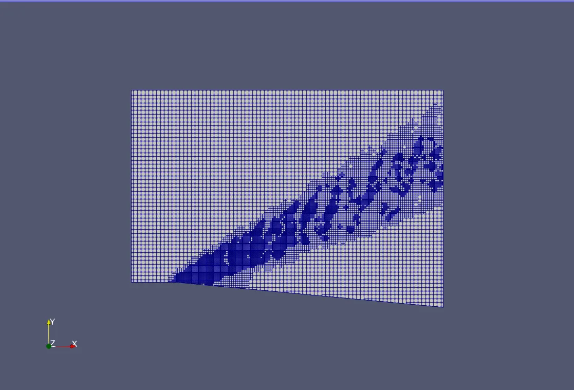
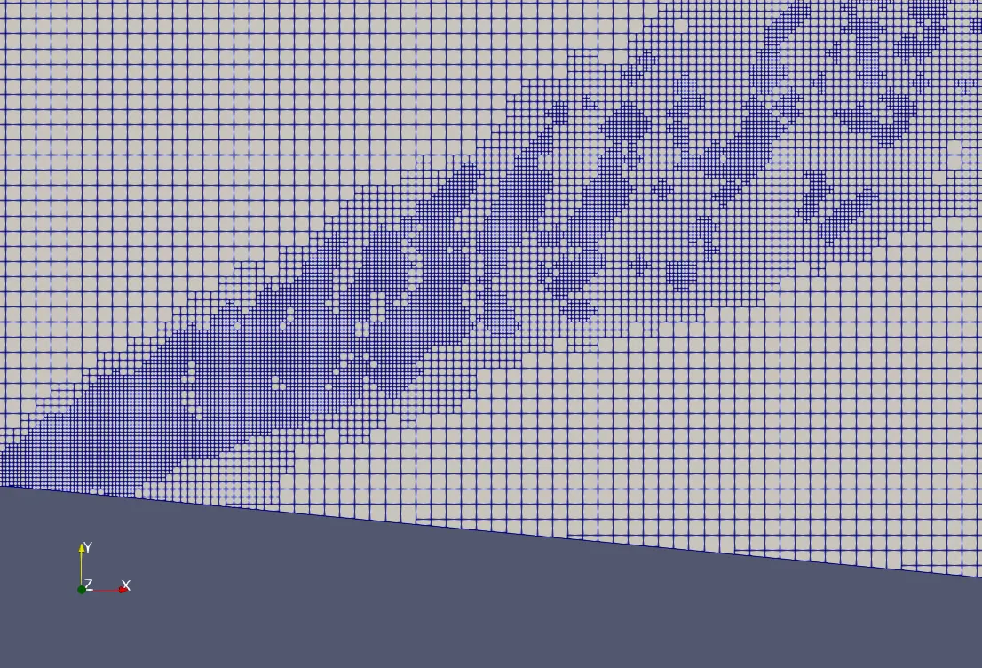
Case Study 2: Grid Size 0.8m SGS 0.01 Velocity 680m/s
Generated Mesh:
Result: (Line Plots & Contours):
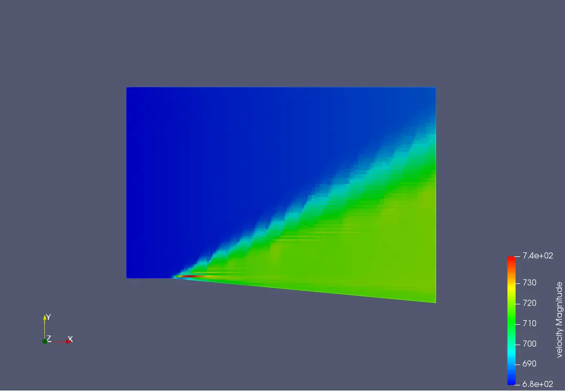
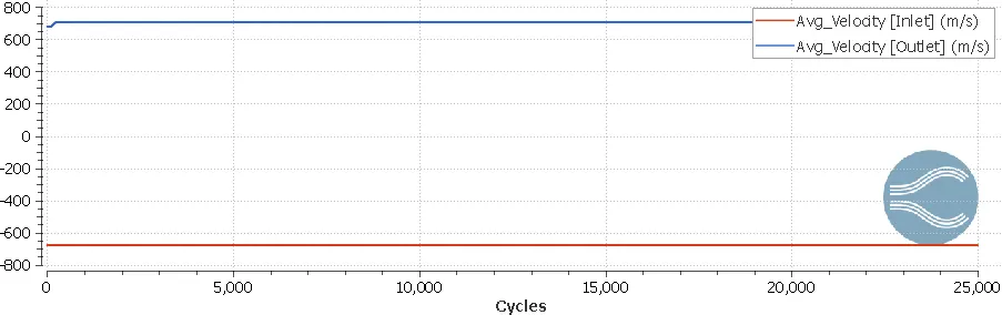
1)Velocity contour and Plot:
2)Pressure Contour and plot:
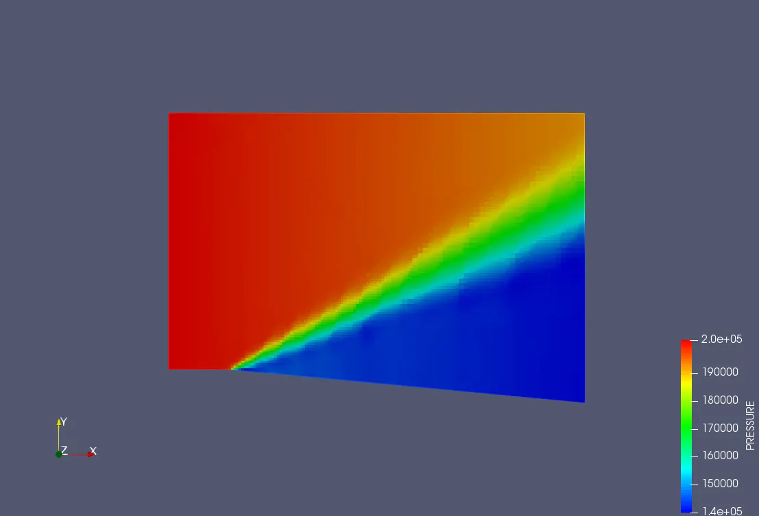
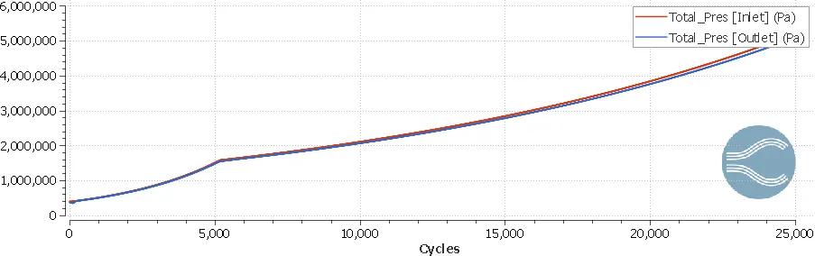
3)Temperature Contour and plot:
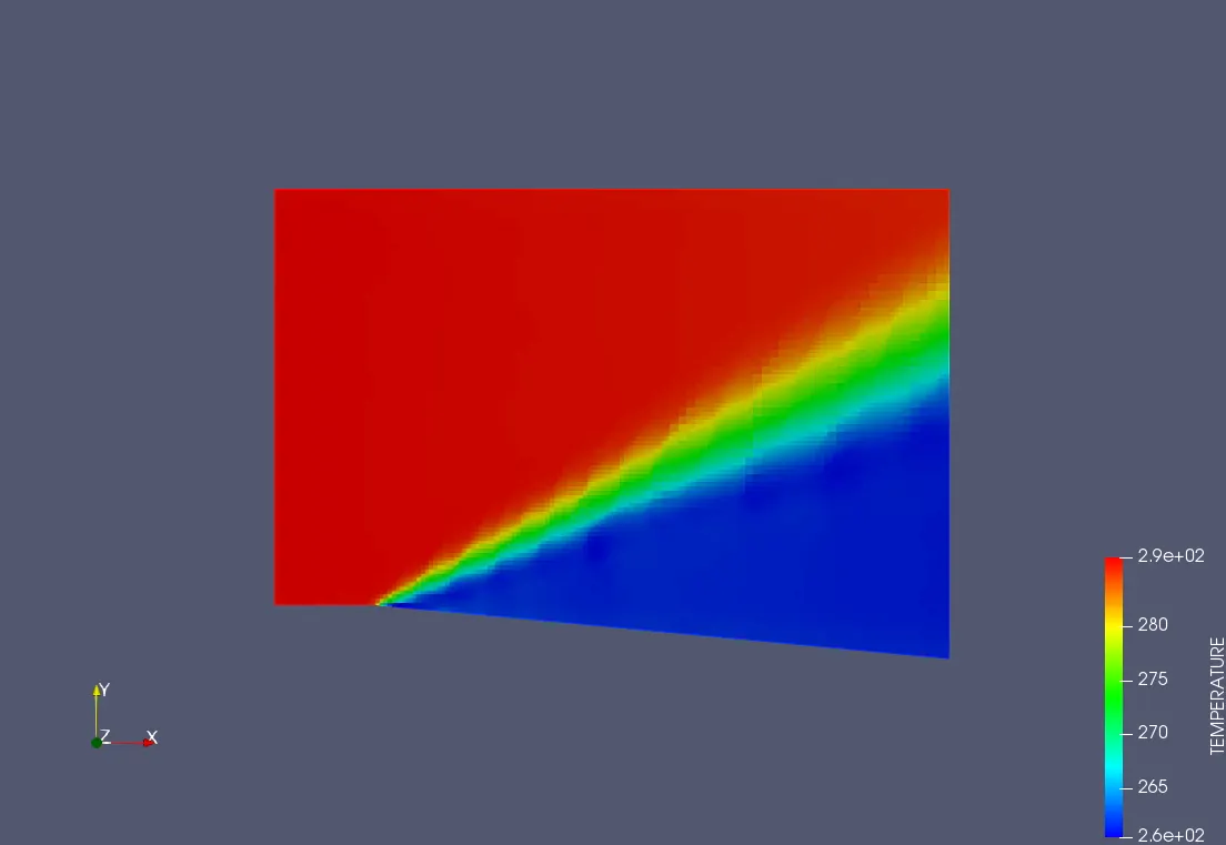
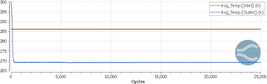
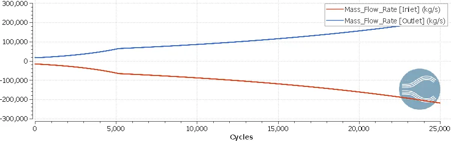
4)Average Mass Flow:
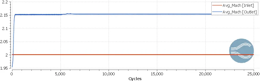
5)Average Mach Number:
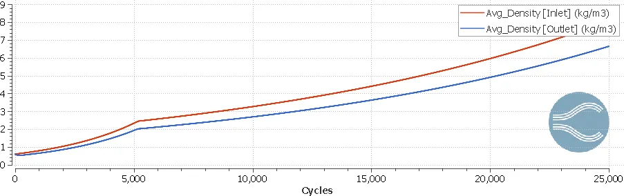
6)Average Density:
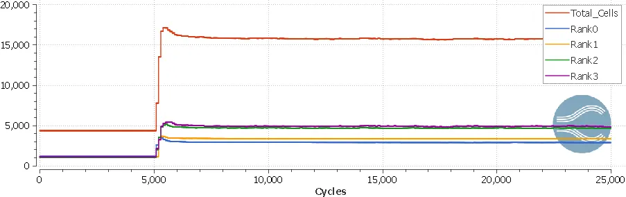
7)Total Cells:
The Youtube link for the animation of velocity,temperature and pressure contours are given below,
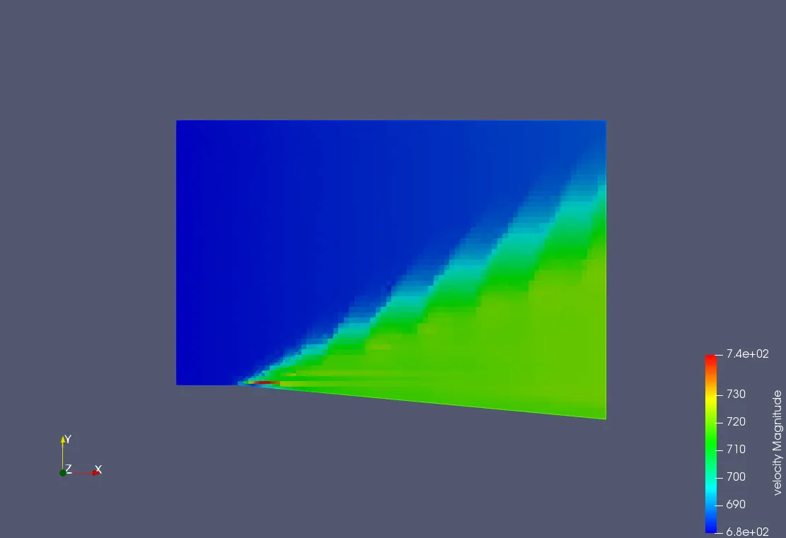
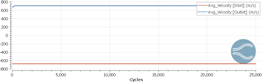
Case Study 3: Grid Size 0.8m SGS 0.1 Velocity 680m/s
Generated Mesh:
Result: (Line Plots & Contours):
1)Velocity contour and Plot:
2)Pressure Contour and plot:
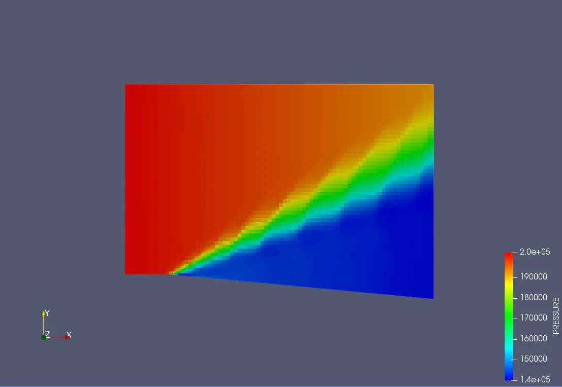
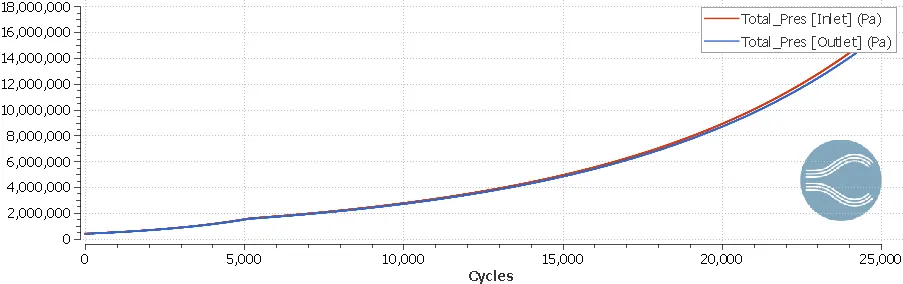
3)Temperature Contour and plot:
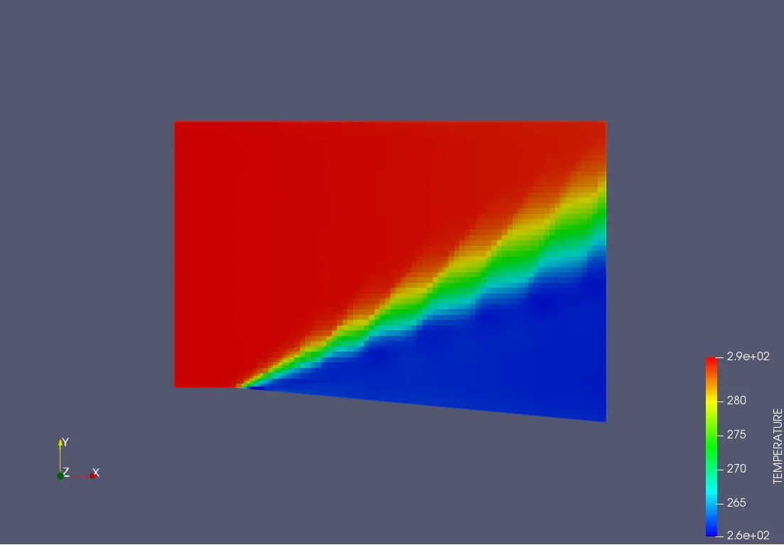
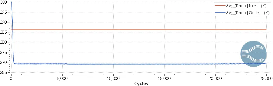
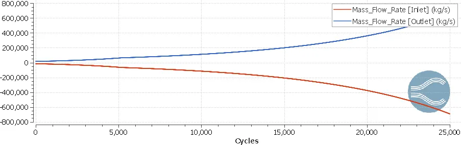
4)Average Mass Flow:
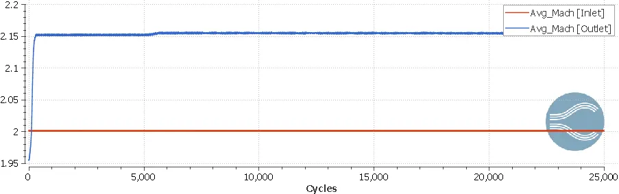
5)Average Mach Number:
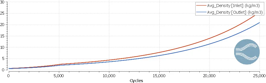
6)Average Density:
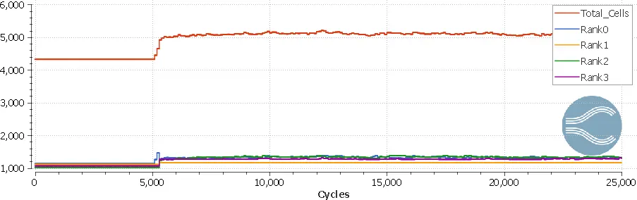
7)Total Cells:
The Youtube link for the animation of velocity,temperature and pressure contours are given below,
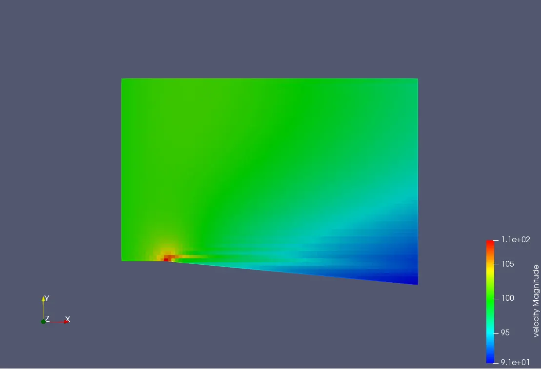
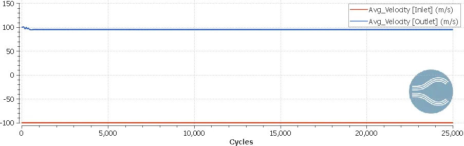
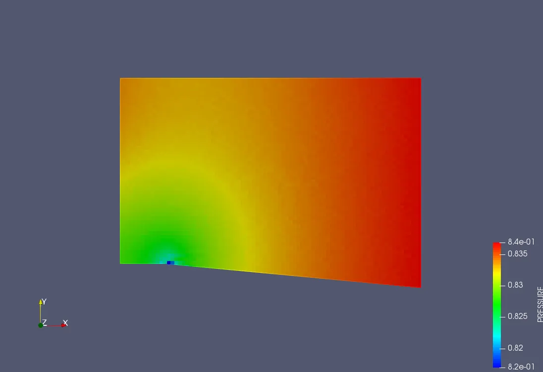
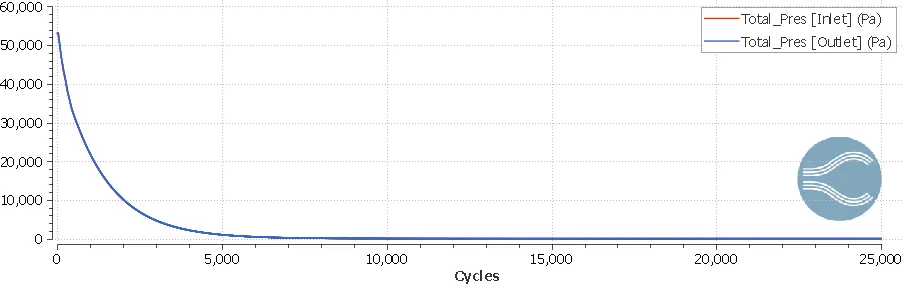
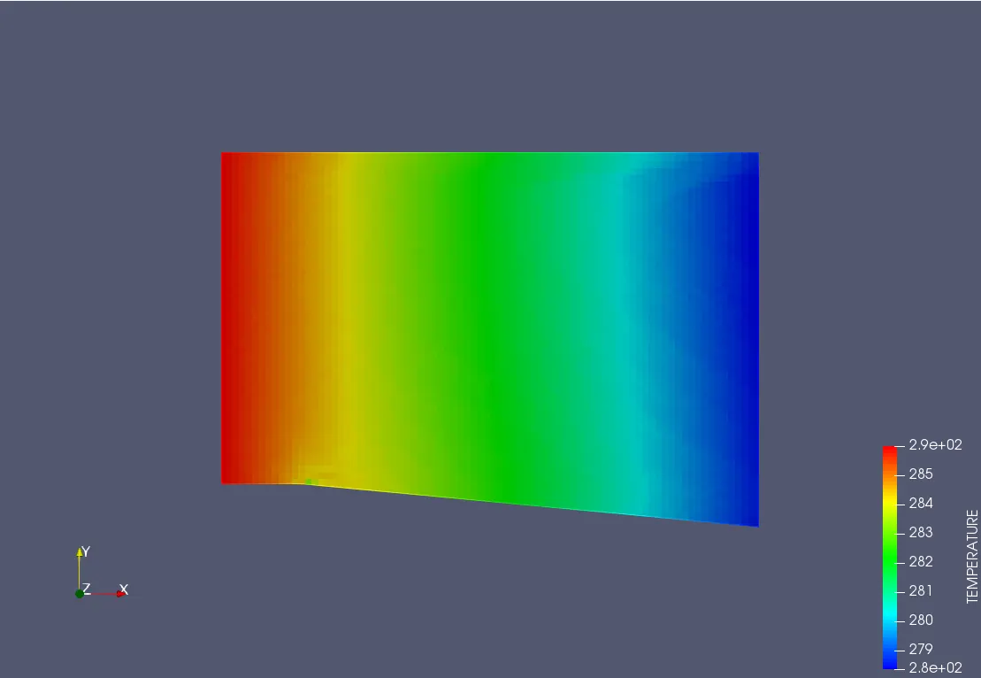
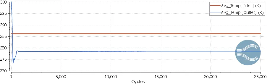
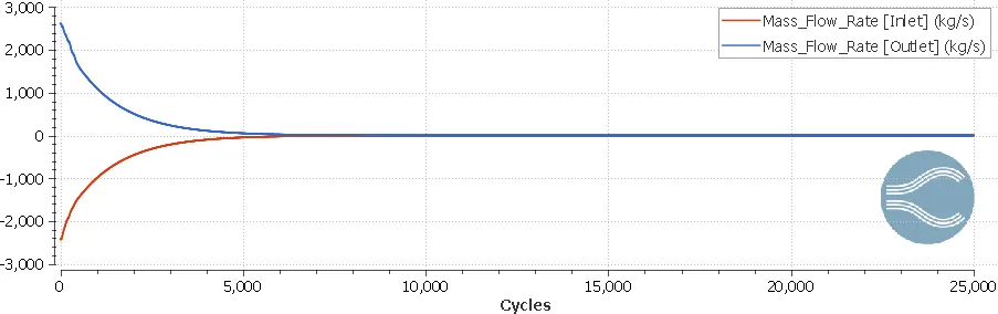
Case Study 4: Grid Size 0.8m SGS 0.05 Velocity 100m/s (Subsonic Flow)
Generated Mesh:
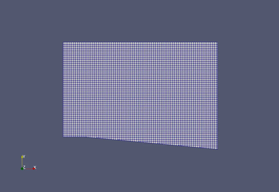
Result: (Line Plots & Contours):
1)Velocity contour and Plot:
2)Pressure Contour and plot:
3)Temperature Contour and plot:
4)Average Mass Flow:
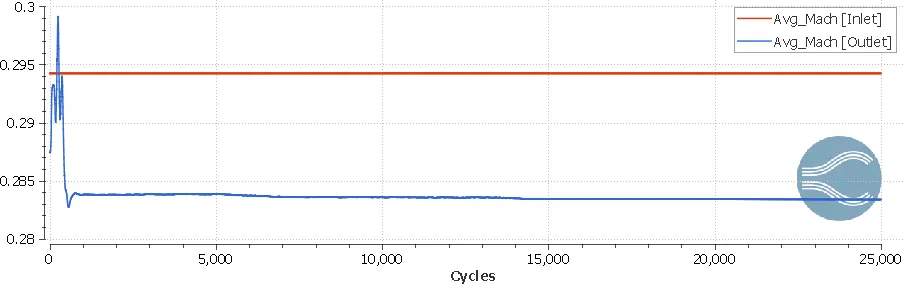
5)Average Mach Number:
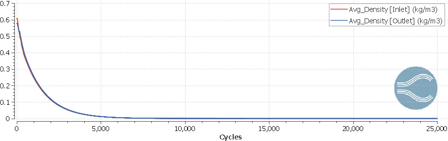
6)Average Density:
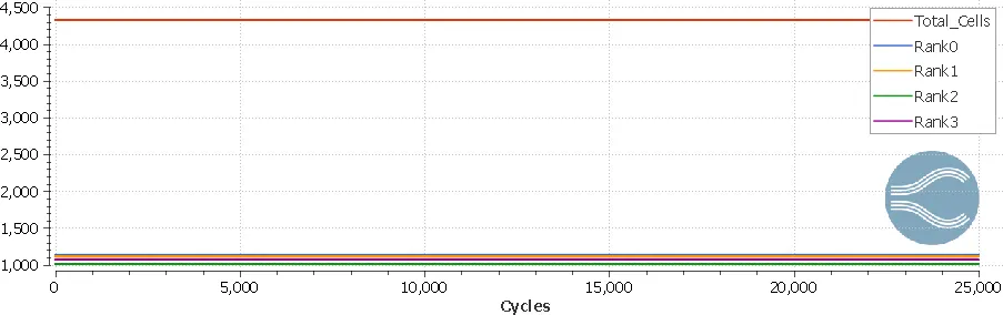
7)Total Cells:
The Youtube link for the animation of velocity,temperature and pressure contours are given below,
Conclusion:
Many things can be noted when we change the value of SGS and inlet velocity.
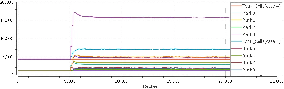
1. Cell count:
Decrease in the SGS parameter, the cell count also increases to capture more data. can be seen from this plot.
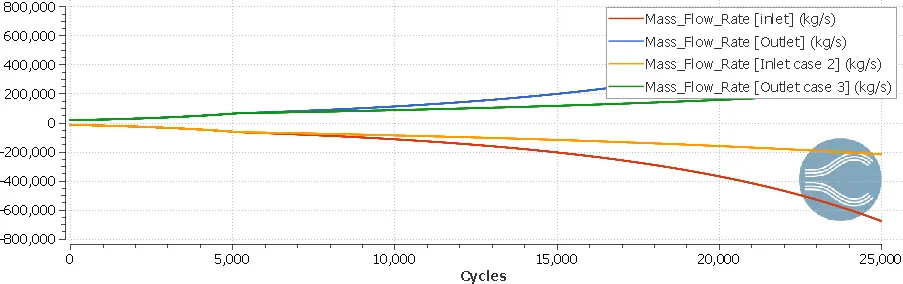
2.Mass Flow Rate:
As the SGS decreases, There is increase in mass flow rate and can be compared using this plot.
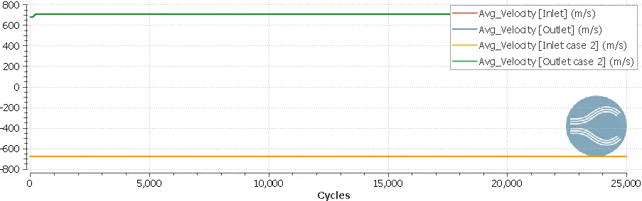
3.Shock location:
For the high SGS parameter, there is coarse quality mesh, and the smaller the value of SGS the mesh quality improves, Hence it affects the value of the case studies that can be seen in these plots.
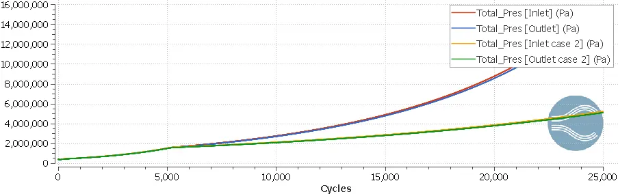
4.Total pressure Comparison:
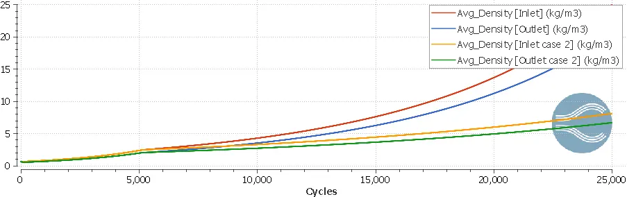
5.Density Comparison for two different cases:
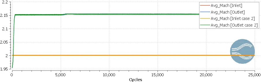
6.Mach number for two different cases:
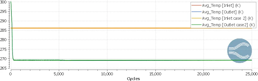
7. Temperature Comparison for two different cases:
Supersonic V/S Subsonic Flow Comparison
In supersonic flow, as we already know that the match number of the flow is just twice a Prandtl-Meyer expansion fan can be seen near to sharp corner which is responsible for generating the shock waves and this area can we improved by reducing the value of SGS parameter in order to capture more cells.
Whereas on the other hand, in subsonic flow, there is not the formation of shock waves even after changing the SGS factor so at last, it can be concluded that the Prandtl-Meyer expansion fan occurs when the speed of flow is more than the speed of sound ie. 340m/s
The Case Study can be download from here Case setup